This blog post will create a simple version of the spectral clustering algorithm for clustering data points. Clustering is one example of an unsupervised task. The algorithm will explore the data in a clustering task and detect some hidden structures. So, there is no target variable to predict.

Introduction

Spectral clustering will cluster our data into groups and find some patterns from even the complex data structure.

Here are some math notations we will use later in this blog:

• Boldface capital letters like \(\mathbf{A}\) refer to matrices (2d arrays of numbers).
• Boldface lowercase letters like \(\mathbf{v}\) refer to vectors (1d arrays of numbers).
• \(\mathbf{A}\mathbf{B}\) refers to a matrix-matrix product (A@B). \(\mathbf{A}\mathbf{v}\) refers to a matrix-vector product (A@v).

First, let’s import the required modules at begining for convenience, then, we can look at an example where we don’t need spectral clustering.

import numpy as np
from sklearn import datasets
from matplotlib import pyplot as plt

Let’s use the function make_blobs() to create two well-separated “blobs” of data. The variable y contains the label to each data point.

n = 200
np.random.seed(1111)
X, y = datasets.make_blobs(n_samples=n, shuffle=True, random_state=None, centers = 2, cluster_std = 2.0)
plt.scatter(X[:,0], X[:,1])

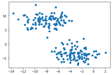
From the above plot, we can notice two circular-ish blobs. In this situation, K-means can quickly achieve the cluster task by identifying centroid inside each cluster.

from sklearn.cluster import KMeans
km = KMeans(n_clusters = 2)
km.fit(X)

plt.scatter(X[:,0], X[:,1], c = km.predict(X))

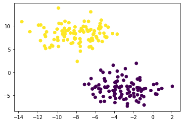
The K-means algorithm clearly partitioned two unlabeled data.

Harder Clustering

The k-means achieve an excellent result when our data are roughly circular; however, K-means perform not well when our data is shaped weirdly.

In the following example, we will explore some uncircular data to check k-means clustering performance.

np.random.seed(1234)
n = 200
X, y = datasets.make_moons(n_samples=n, shuffle=True, noise=0.05, random_state=None)
plt.scatter(X[:,0], X[:,1])

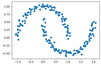
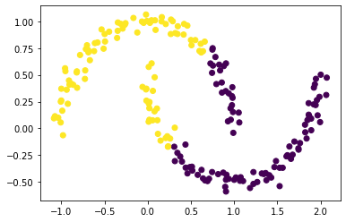
The above plot still shows two possible clusters of data with crescents shapes.. As before, the Euclidean coordinates of the data points are contained in the matrix X, while the labels of each point are contained in y. Now k-means won’t work so well, because k-means is, by design, looking for circular clusters.

km = KMeans(n_clusters = 2)
km.fit(X)
plt.scatter(X[:,0], X[:,1], c = km.predict(X))

Part A: Similarity Matrix

Before we use spectral clustering, we need to construct the similarity matrix \(\mathbf{A}\). \(\mathbf{A}\) should be a square matrix with the shape (n, n) with n number of data points.

We use the idea of a similarity graph to construct the similarity matrix. First, we can connect all data points and find all pairwise distances. We define whether any two points are connected if those two points are within distance ε. If any of two points are connected ((i, j) < ε), we set A[i, j] = 1, otherwise A[i, j] =0. Also, we should have a similarity matrix with diagonal entries are equal to zero.

We will use function pairwise_distances() from the sklearn.metrics package to compute the required similarity matrix.

# https://scikit-learn.org/stable/modules/metrics.html#metrics
from sklearn.metrics import pairwise_distances

epsilon = 0.4

# change boolean matrix to numbers
A = (pairwise_distances(X, X, metric='euclidean') < epsilon) + 0 
np.fill_diagonal(A, 0)   # make sure diagonal are 0
A

array([[0, 0, 0, ..., 0, 0, 0],
       [0, 0, 0, ..., 0, 0, 0],
       [0, 0, 0, ..., 0, 1, 0],
       ...,
       [0, 0, 0, ..., 0, 1, 1],
       [0, 0, 1, ..., 1, 0, 1],
       [0, 0, 0, ..., 1, 1, 0]])

Part B: The Cut and Volume Term

Now, our similarity matrix A can tell us which points are connected. We now pose the task of clustering the data points in X as the task of partitioning the rows and columns of A.

Let \(d_i = \sum_{j = 1}^n a_{ij}\) be the \(i\)th row-sum of \(\mathbf{A}\), which is also called the degree of \(i\).

Let \(C_0\) and \(C_1\) be two clusters of the data points. We assume that every data point is in either \(C_0\) or \(C_1\).

The cluster membership as being specified by y. We think of y[i] as being the label of point i. So, if y[i] = 1, then point i (and therefore row \(i\) of \(\mathbf{A}\)) is an element of cluster \(C_1\).

The binary norm cut objective of a matrix \(\mathbf{A}\) is the function

In this expression,

• \(\mathbf{cut}(C_0, C_1) \equiv \sum_{i \in C_0, j \in C_1} a_{ij}\) is the cut of the clusters \(C_0\) and \(C_1\).
• \(\mathbf{vol}(C_0) \equiv \sum_{i \in C_0}d_i$, where $d_i = \sum_{j = 1}^n a_{ij}\) is the degree of row \(i\) (the total number of all other rows related to row \(i\) through \(A\)). The volume of cluster \(C_0\) is a measure of the size of the cluster.

A pair of clusters \(C_0\) and \(C_1\) is considered to be a “good” partition of the data when \(N_{\mathbf{A}}(C_0, C_1)\) is small. To see why, let’s look at each of the two factors in this objective function separately.

B.1 The Cut Term

The cut term shows how two labels are associated.

If we have a small cut term, which means we do not have too much connection between our two clusters \(C_0\) and \(C_1\).

Next, we will write a function cut(A,y) to obtain the cut term.

def cut(A, y):
    """
    This function will find the number of cut term of A
    by summing up the entries A[i, j] 
    for each pair of points (i,j) in different clusters.
    """
    num_cut = 0
    
    # loop over each different pair of points in y
    for i in range(len(y)):
        for j in range(i, len(y)):
            if y[i]!=y[j]:         # check if they are in different clusters  
                num_cut += A[i,j] 
                
    return num_cut 

In the next cell, we will compute the two cut objectives. One is for the actual clusters y, and another is a random vector of random labels of length n, with each label equal to either 0 or 1.

Then we will compare these cut objectives.

cut_true = cut(A,y)                          #  cut objective for the true clusters y
random_y = np.random.randint(0,2, size = n)  # a random vector of random labels of length n
cut_random = cut(A, random_y)                # cut objective for the random labels

print("cut objective for the true labels:   " + str(cut_true))
print("cut objective for the random labels: " + str(cut_random))

cut objective for the true labels:   13
cut objective for the random labels: 1150

We noticed from the above result that the number of cut objectives is much smaller than the random ones.

B.2 The Volume Term

Our second factor is the norm cut objective which is also the volume term.

A volume of a cluster tells us the size of that cluster. Notice that, If we choose cluster \(C_0\) to be small, then \(\mathbf{vol}(C_0)\) will be small and \(\frac{1}{\mathbf{vol}(C_0)}\) will be large, leading to an undesirable higher objective value.

To find the binary normcut objective, we need to find clusters \(C_0\) and \(C_1\) such that:

1. There are relatively few entries of \(\mathbf{A}\) that join \(C_0\) and \(C_1\).
2. Neither \(C_0\) and \(C_1\) are too small.

def vols(A, y):
    """
    This function will computes the volumes of C0 and C1, returning them as a tuple. 
    (volume of cluster `0`, volume of cluster `1`) 
    """
    return ((sum(A.sum(axis= 0)[y==0])), (sum(A.sum(axis= 0)[y==1])))


def normcut(A, y):
    """
    This function uses cut(A,y) and vols(A,y) 
    to compute the binary normalized cut objective of a matrix A with clustering vector y.
    """
    v0, v1 = vols(A, y)
    return (cut(A, y) * ((1/v0) + (1/v1)))

First, let’s compute the normcut objective using the true labels y.

normcut(A, y)

0.011518412331615225

Then, let’s compute the normcut objective using the fake labels we generated before.

normcut(A, random_y)

1.0240023597759158

Comparing the above two results of our normcut objective, we can see that the normcut objective using the true label y is significantly smaller than the normcut objective using the fake labels we generated before.

Part C: Transform

One method to clustering from a normalized cut objective is to try to find a cluster vector y such that normcut(A,y) is small. But, using this method is not efficient; it might not be possible to find the best clustering in practical time, even for relatively small data sets. So, we need a math trick to solve this problem.

First, we should define a new vector \(\mathbf{z} \in \mathbb{R}^n\) such that:

Note that the signs of the elements of \(\mathbf{z}\) contain all the information from \(\mathbf{y}\): if $i$ is in cluster \(C_0\), then \(y_i = 0\) and \(z_i > 0\).

Next, if you like linear algebra, you can show that

where \(\mathbf{D}\) is the diagonal matrix with nonzero entries \(d_{ii} = d_i\), and where \(d_i = \sum_{j = 1}^n a_i\) is the degree (row-sum) from before.

The first step is that we should write the transform(A,y) function to compute the appropriate \(\mathbf{z}\) vector given A and y, using the formula: \(z_i = \begin{cases} \frac{1}{\mathbf{vol}(C_0)} &\quad \text{if } y_i = 0 \\ -\frac{1}{\mathbf{vol}(C_1)} &\quad \text{if } y_i = 1 \\ \end{cases}\)

def transform(A, y):
    """
    This function computes the appropriate z vector which contain all the information from y 
    by givening A and y, using the formula above.
    """
    v0, v1 = vols(A, y)
    z = np.ones(len(y))/v0
    z[y==1] = -1/v1
    
    return z
    

Then, we should check that each side of the equation \(\mathbf{N}_{\mathbf{A}}(C_0, C_1) = \frac{\mathbf{z}^T (\mathbf{D} - \mathbf{A})\mathbf{z}}{\mathbf{z}^T\mathbf{D}\mathbf{z}}\;,\) is equal by using the function normcut(A, y) and matrix product.

z = transform(A, y)              # z vector
D = np.diag(A.sum(axis=0))       # diagonal matrix with nonzero entries

check1 = normcut(A, y)           #   using function normcut()
check2 = ((z@(D-A)@z)/(z@D@z))   #   using matrix product

print(check1)
print(check2)
print(np.isclose(check1, check2))

0.011518412331615225
0.011518412331615099
True

Let’s also check the identity \(\mathbf{z}^T\mathbf{D}\mathbb{1} = 0\), where \(\mathbb{1}\) is the vector of n ones. This identity effectively says that \(\mathbf{z}\) should contain roughly as many positive as negative entries.

v_one = np.ones(n)
np.isclose(z.T@D@v_one, 0)

True

Great, we have successfully constructed the new vector \(\mathbf{z}\).

Part D: Minimizing the Function

In the last part, we saw that the problem of minimizing the normcut objective is mathematically related to the problem of minimizing the function

subject to the condition \(\mathbf{z}^T\mathbf{D}\mathbb{1} = 0\). It’s actually possible to bake this condition into the optimization, by substituting for \(\mathbf{z}\) the orthogonal complement of \(\mathbf{z}\) relative to \(\mathbf{D}\mathbf{1}\).

In the next cell, let’s define an orth_obj function which find the orthogonal complement of \(\mathbf{z}\) relative to \(\mathbf{D}\mathbf{1}\).

def orth(u, v):
    return (u @ v) / (v @ v) * v

e = np.ones(n) 

d = D @ e

def orth_obj(z):
    z_o = z - orth(z, d)
    return (z_o @ (D - A) @ z_o)/(z_o @ D @ z_o)

Next we find the minimizing vector z_min by using the minimize function from scipy.optimize to minimize the function orth_obj() with respect to \(\mathbf{z}\).

scipy.optimize.minimize(fun, x0), x0 is initial guess.

from scipy.optimize import minimize

# using the initial guess a vector of random numbers between -1 and 
# let's use the randome numbers from 0 to 1
guess = np.random.random(n)

# The optimization result represented as a OptimizeResult object.
# Important attributes are: x the solution array
z_min = minimize(orth_obj, guess).x 

Part E: Clustering with Minimizing Vector

The sign of z_min[i] contains information about the cluster label of data point i.

• \(y_i = 0\) and \(z_i > 0\), \(i\) is in cluster \(C_0\)
• \(y_i = 1\) and \(z_i < 0\), \(i\) is in cluster \(C_1\)

Finally, we can plot our original “shaped weird” data.

plt.scatter(X[:,0], X[:,1], c = z_min<0)

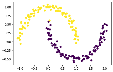
The result looks pretty great; it clearly shows two groups of data.

Part F: Laplacian Matrix

Maybe you wonder if there is an even faster approach than explicitly optimizing. Luckily, we can try to find the eigenvector corresponding to its second-smallest eigenvalue in the Laplacian or normalized matrix \(\mathbf{L} = \mathbf{D}^{-1}(\mathbf{D} - \mathbf{A})\) .

L = np.linalg.inv(D)@(D-A)  # Laplacian or normalized matrix

Lam_eigenvalues, U_eigenvector = np.linalg.eig(L) # compute the eigenvalues and eigenvectors of L

ix = Lam_eigenvalues.argsort() # get the indices that would sort our eigenvalues

Lam_eigenvalues, U_eigenvector = Lam_eigenvalues[ix],  U_eigenvector[:, ix]

# second-smallest eigenvalue
z_eig = U_eigenvector[:, 1]

Now, we can plot our original “shaped weird” data again by using our new approach with the second-smallest eigenvalue z_eig. We also used the color associated with the sign of z_eig.

# The sign function returns -1 if x < 0, 0 if x==0, 1 if x > 0

plt.scatter(X[:,0], X[:,1], c = np.sign(z_eig))

The result looks great too, and using the z_eig approach is way faster than using the z_min approach.

Part G: Synthesize the Results

In this part, we will wrap all our previously defined functions into one function called spectral_clustering(X, epsilon) to performs spectral clustering; This function accepts two arguments: X (the Euclidean coordinates of the data points) and epsilon (the distance threshold).

def spectral_clustering(X, epsilon):
    """
    This function will performs spectral clustering of the data
    
    Parameters
    ----------
    X: np.ndrray; the Euclidean coordinates of the data points
                  In our case, X has shape (200, 2)
    epsilon: float; the distance threshold
    
    Return
    ----------
    ((z_eig>0)+0): an array of binary labels indicating whether data point i is in group 0 or group 1
    
    """
    
    # Construct the similarity matrix
    A = (pairwise_distances(X, X, metric='euclidean') < epsilon) + 0 
    np.fill_diagonal(A, 0)    # make sure diagonal are 0
    
    # Construct the Laplacian matrix
    D = np.diag(A.sum(axis=0))
    L = np.linalg.inv(D)@(D-A)
    
    # Compute the eigenvector with second-smallest eigenvalue of the Laplacian matrix
    Lam_eigenvalues, U_eigenvector = np.linalg.eig(L)
    ix = Lam_eigenvalues.argsort()
    Lam_eigenvalues, U_eigenvector = Lam_eigenvalues[ix],  U_eigenvector[:, ix]
    z_eig = U_eigenvector[:, 1]

    # Return labels based on this second-smallest eigenvector
    return ((z_eig>0)+0)

Let’s use our function spectral_clustering(X, epsilon) to make the plot again from our original “shaped weird” data.

plt.scatter(X[:,0], X[:,1], c = spectral_clustering(X, epsilon))

Part H: More Experiments

In this section, we will do a few more experiments with n = 1000 datapoints using the function spectral_clustering(X, epsilon) with a different dataset generated by the function datasets.make_moons(); Then, we will explore the parameter noise with various numbers inside the function datasets.make_moons().

n = 1000
X, y = datasets.make_moons(n_samples=n, shuffle=True, noise=0.06, random_state=None)
plt.scatter(X[:,0], X[:,1], c = spectral_clustering(X, epsilon))

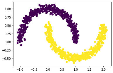
When we have a smaller number of noise, our spectral clustering function works perfectly.

let’s try noise = 0.1.

n = 1000
X, y = datasets.make_moons(n_samples=n, shuffle=True, noise=0.1, random_state=None)
plt.scatter(X[:,0], X[:,1], c = spectral_clustering(X, epsilon))

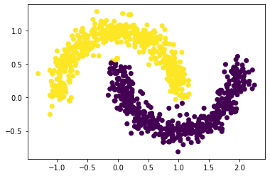
Our spectral clustering function still did a good job when we increased the noise to 0.1.

let’s try noise = 0.2

n = 1000
X, y = datasets.make_moons(n_samples=n, shuffle=True, noise=0.2, random_state=None)
plt.scatter(X[:,0], X[:,1], c = spectral_clustering(X, epsilon))

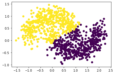
It seems our spectral clustering function does not work in this situation.

As a result, our spectral clustering function performs better when the noise is small.

Part I

Let’s try another fun dataset – the bull’s eye!

n = 1000
X, y = datasets.make_circles(n_samples=n, shuffle=True, noise=0.05, random_state=None, factor = 0.4)
plt.scatter(X[:,0], X[:,1])

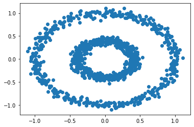
There are two concentric circles. Let’s use k-means to check what we will get.

km = KMeans(n_clusters = 2)
km.fit(X)
plt.scatter(X[:,0], X[:,1], c = km.predict(X))

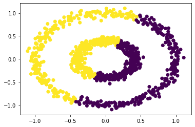
No surprise, since our data are roughly circular, k-means will not perform well in this case.

Let’s try some different values of epsilon between 0 and 1.0.

In the next cell, we can create a function different_epsilon() to create spectral clustering plots of different epsilon values between 0 and 1.0.

import math   

def different_epsilon (epsilon_array, figsize):
    """
    This function will make mutiple subplots from our spectral clustering function
    with different epsilon between 0 and 1.0. 
    
    Parameters
    ----------
    epsilon_array: array; array contains all different epsilon values
    figsize : tuple; size of the figure
    
    Return
    ----------
    No return values 
    """
    
    # change array to list
    epsilon_list = epsilon_array.tolist()
    # make the plot
    fig, axarr = plt.subplots(math.ceil(len((epsilon_list))/4), 4, figsize = figsize)
    
    # loop over each axis
    for ax in axarr.flatten():
        if (epsilon_list):
            epsilon = epsilon_list.pop(0)
            epsilon = round(epsilon,2)
            ax.axis("off")
            ax.set(title = "epsilon = " + str(epsilon))
            ax.scatter(X[:,0], X[:,1], c = spectral_clustering(X, epsilon))
            

# different values of epsilon between 0.2 and 1.0 with step=0.5
different_epsilon(epsilon_array = np.arange(0.2,1,0.05), figsize=(20,10))

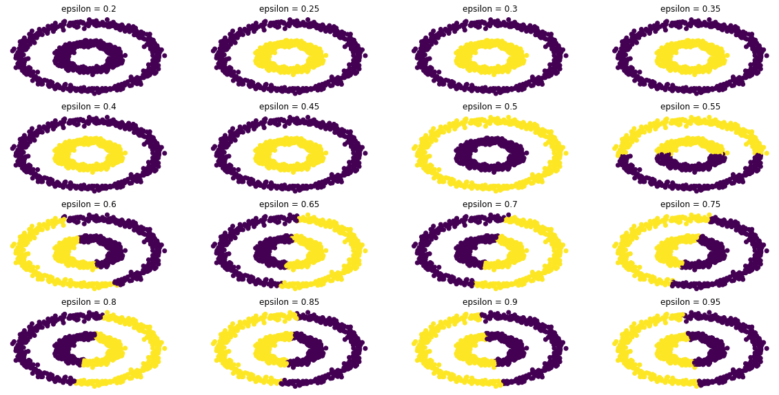
From the above result, we can see that approximately our function can correctly separate the two rings when 0.25 \(\leq\) \(\epsilon\) \(\leq\) 0.5.

However, we can notice that when \(\epsilon\) =0.25; our function still correctly separates the two rings; Let’s make our epsilon even smaller.

different_epsilon(epsilon_array=np.arange(0.15,0.55,0.01), figsize= (20,20))

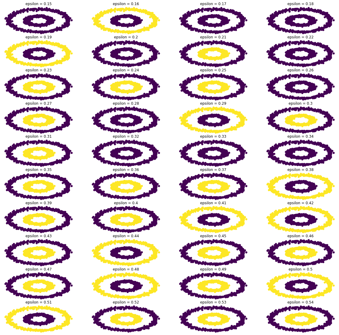
As a result, we are able to separate the two rings roughly when

• 0.35 \(\leq\) \(\epsilon\) \(\leq\) 0.54
• 0.29 \(\leq\) \(\epsilon\) \(\leq\) 0.31
• 0.23 \(\leq\) \(\epsilon\) \(\leq\) 0.25
• \(\epsilon\) = 0.16, 0.19, 0.21