We will use TensorFlow to classify images between dogs or cats in this post. TensorFlow is a Google product, and the tensor is similar to the NumPy array. We should have some basic understanding of neural networks before knowing what TensorFlow is. Neural networks are the operations of matrix multiplication and simple, nonlinear functions.

Here are some useful information from IBM, which shows How do artificial intelligence, machine learning, neural networks, and deep learning relate?

Perhaps the easiest way to think about artificial intelligence, machine learning, neural networks, and deep learning is to think of them like Russian nesting dolls. Each is essentially a component of the prior term.

That is, machine learning is a subfield of artificial intelligence. Deep learning is a subfield of machine learning, and neural networks make up the backbone of deep learning algorithms. In fact, it is the number of node layers, or depth, of neural networks that distinguishes a single neural network from a deep learning algorithm, which must have more than three.

Acknowledgment

Major parts of this Blog Post assignment, including several code chunks, explanations are based on the TensorFlow Transfer Learning Tutorial and from Professor Chodrow.

§1. Load Packages and Obtain Data

I will put all import statements here at beginning for convenience.

import os
import tensorflow as tf
import matplotlib.pyplot as plt
import numpy as np

# from tensorflow.keras Import  utils 
# from tensorflow.keras import layers
# I got some error for import "tensorflow.keras"
# in google colab by using GPU accelerator.
# ex: Import "tensorflow.keras" could not be resolved
# so i will use tf.keras.utils and tf.keras.layers
# instead of importing utils and layers from tensorflow.keras

In this section, we will download the required sample data from the TensorFlow team. This dataset contains many labeled images of cats and dogs. After we load our image datasets we will use the method tf.keras.utils.image_dataset_from_directory() to generates tf.data.Dataset object for our training and validation datasets. Then we will take every 5th observation out of the validation dataset as our test datasets.

# location of data
_URL = 'https://storage.googleapis.com/mledu-datasets/cats_and_dogs_filtered.zip'

# download the data and extract it
path_to_zip = tf.keras.utils.get_file('cats_and_dogs.zip', origin=_URL, extract=True)

# construct paths
PATH = os.path.join(os.path.dirname(path_to_zip), 'cats_and_dogs_filtered')

train_dir = os.path.join(PATH, 'train')
validation_dir = os.path.join(PATH, 'validation')

# parameters for datasets
BATCH_SIZE = 32
IMG_SIZE = (160, 160)

# construct train and validation datasets 
train_dataset = tf.keras.utils.image_dataset_from_directory(train_dir,
                                                   shuffle=True,
                                                   batch_size=BATCH_SIZE,
                                                   image_size=IMG_SIZE)

validation_dataset = tf.keras.utils.image_dataset_from_directory(validation_dir,
                                                        shuffle=True,
                                                        batch_size=BATCH_SIZE,
                                                        image_size=IMG_SIZE)
class_names = train_dataset.class_names

# construct the test dataset by taking every 5th observation out of the validation dataset
val_batches = tf.data.experimental.cardinality(validation_dataset)
test_dataset = validation_dataset.take(val_batches // 5)
validation_dataset = validation_dataset.skip(val_batches // 5)

Found 2000 files belonging to 2 classes.
Found 1000 files belonging to 2 classes.

We have successfully created TensorFlow Datasets for training, validation, and testing. We’ve used a special-purpose keras utility called image_dataset_from_directory to construct a Dataset. The first argument indicates the directory where the data is located. Next, we set shuffle argument True to get the randomized images. We let batch_size argument equals 32 which means our algorithm takes 32 images each time from the directory. If we higher the batch_size, more computer memory needed. The argument image_size resize the input images to dimension (160,160), since the pipeline processes batches of images requires the same size of images.

The next block of code is technical code related to rapidly reading data, click here to know more.

The tf.data API provides the tf.data.Dataset.prefetch transformation. It can be used to decouple the time when data is produced from the time when data is consumed. In particular, the transformation uses a background thread and an internal buffer to prefetch elements from the input dataset ahead of the time they are requested. The number of elements to prefetch should be equal to (or possibly greater than) the number of batches consumed by a single training step. You could either manually tune this value, or set it to tf.data.AUTOTUNE, which will prompt the tf.data runtime to tune the value dynamically at runtime.

AUTOTUNE = tf.data.AUTOTUNE

train_dataset = train_dataset.prefetch(buffer_size=AUTOTUNE)
validation_dataset = validation_dataset.prefetch(buffer_size=AUTOTUNE)
test_dataset = test_dataset.prefetch(buffer_size=AUTOTUNE)

Working with Datasets

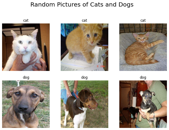
In the next cell, we will write the function two_row_visualization()to randomly show three images of cats in the first row and three random images of dogs in the second row. Note: Cat is encoded as 0; Dog is 1.

def two_row_visualization():
  """
  This function will show three random pictures of cats in the first row;
  and show three random pictures of dogs in the second row.
  """

  plt.figure(figsize=(10, 10))
  plt.suptitle("Random Pictures of Cats and Dogs", fontsize=20)
  # loop over one batch of 32 images with labels from the training data
  for images, labels in train_dataset.take(1):
    # change labels tensor object to numpy array 
    labels_array = labels.numpy()
    # randomly pick three indexes of cat images
    cat_index = (np.random.choice(np.where(labels_array == 0)[0], 3, replace=False))
    # randomly pick three indexes of dog images
    dog_index = (np.random.choice(np.where(labels_array == 1)[0], 3, replace=False))
    # the first three indexes are cat, last three are dog
    cat_dog = (np.concatenate((cat_index, dog_index)))
    # loop over 6 images
    for i in range(6):
      ax = plt.subplot(3, 3, i+1)
      plt.imshow(images[cat_dog[i]].numpy().astype("uint8"))
      # set title for cat or dog
      plt.title(["cat" if labels_array[cat_dog[i]]==0 else "dog"][0])
      plt.axis("off")
    

Let’s explore our dataset by using our function two_row_visualization().

two_row_visualization()

Check Label Frequencies

The following line of code will create an iterator called labels.

labels_iterator= train_dataset.unbatch().map(lambda image, label: label).as_numpy_iterator()

Next, we will caculate total number of images and how many are cats.

• label 0 is cat
• label 1 is dog

labels_list = list(labels_iterator)
print("Totoal number of images: " + str(len(labels_list)))
print("Total number of cats: " + str(labels_list.count(0)))

Totoal number of images: 2000
Total number of cats: 1000

Now, we can use the above information to find out our baseline machine learning model.

Since we have 1000 images of cat out of a total of 2000 images, our images datasets are well balanced. Therefore, we expected the accuracy of the baseline model should be at least 0.5.

§2. First Model

In this section, we will build our first machine learning model. We will use the simplest way to make our first model using the tf.keras.Sequential API, which allows us to construct a model by simply passing a list of layers.

• Kernel is a matrix that can help us to extract features from images.

• Conv2D Layer: create a layer of user-specified convolutional kernels. Larger kernels can extract more complicated information, but it takes longer to learn since it increases the complexity of computing them.

• MaxPooling2D Layer : pooling layers act as “summaries” that reduce the data size at each step. Max pooling involves sliding a window over the current batch of data and picking only the largest element within that window.

• Flatten Layer : flatten the data from 2D to 1D in order to pass the final Dense layer.

• Dense Layer : a dense layer is the simplest, and among the most generally useful layers The Dense layer interprets an m x n tensor as a set of data points with m rows and n columns (or features).

• Dropout Layer: dropout layer will disable a fixed percentage of the units in each layer, but only during training. Using this layer is a good way to reduce the risk of overfitting.

Next, we will create a function called history_plot(), which will plot the history of the accuracy on both the training and validation sets.

def history_plot():
  """
  This function will create the plot of accuracy on the training and validation sets
  """
  plt.figure(figsize=(10,5))
  plt.plot(history.history["accuracy"], label = "training")
  plt.plot(history.history["val_accuracy"], label = "validation")
  plt.gca().set(xlabel = "epoch", ylabel = "accuracy")
  plt.title("Training and Validation Performance")
  plt.legend()

It’s time to build our first model now.

model1 = tf.keras.Sequential([               
      tf.keras.layers.Conv2D(32, (3, 3), activation='relu', input_shape=(160, 160, 3)),
      tf.keras.layers.MaxPooling2D((2, 2)),
      tf.keras.layers.Conv2D(32, (3, 3), activation='relu'),
      tf.keras.layers.MaxPooling2D((2, 2)),
      tf.keras.layers.Conv2D(64, (3, 3), activation='relu'),
      tf.keras.layers.MaxPooling2D((2, 2)),
      tf.keras.layers.Dropout(0.2),
      tf.keras.layers.Conv2D(64, (3, 3), activation='relu'),
      tf.keras.layers.MaxPooling2D((2, 2)),
      tf.keras.layers.Flatten(),
      tf.keras.layers.Dense(128, activation='relu'),
      tf.keras.layers.Dropout(0.2),
      tf.keras.layers.Dense(2, activation="softmax") # number of classes
     
])

model1.compile(optimizer="adam",
              loss=tf.keras.losses.SparseCategoricalCrossentropy(),
              metrics=['accuracy'])

history = model1.fit(train_dataset,
                    epochs=20, 
                    validation_data=validation_dataset)

I will show the last training epoch here:

Epoch 20/20
63/63 [==============================] - 5s 70ms/step - loss: 0.1192 - accuracy: 0.9550 - val_loss: 1.6240 - val_accuracy: 0.6312

    Epoch 1/20
    63/63 [==============================] - 14s 68ms/step - loss: 3.8792 - accuracy: 0.5225 - val_loss: 0.6928 - val_accuracy: 0.5235
    Epoch 2/20
    63/63 [==============================] - 4s 64ms/step - loss: 0.6890 - accuracy: 0.5375 - val_loss: 0.6855 - val_accuracy: 0.5941
    Epoch 3/20
    63/63 [==============================] - 4s 64ms/step - loss: 0.6905 - accuracy: 0.5500 - val_loss: 0.6785 - val_accuracy: 0.5594
    Epoch 4/20
    63/63 [==============================] - 4s 66ms/step - loss: 0.6722 - accuracy: 0.5715 - val_loss: 0.6597 - val_accuracy: 0.6114
    Epoch 5/20
    63/63 [==============================] - 4s 66ms/step - loss: 0.6404 - accuracy: 0.6250 - val_loss: 0.6593 - val_accuracy: 0.6213
    Epoch 6/20
    63/63 [==============================] - 4s 67ms/step - loss: 0.5994 - accuracy: 0.6695 - val_loss: 0.6629 - val_accuracy: 0.6015
    Epoch 7/20
    63/63 [==============================] - 4s 64ms/step - loss: 0.5753 - accuracy: 0.6975 - val_loss: 0.6692 - val_accuracy: 0.6399
    Epoch 8/20
    63/63 [==============================] - 4s 65ms/step - loss: 0.5416 - accuracy: 0.7130 - val_loss: 0.6359 - val_accuracy: 0.6609
    Epoch 9/20
    63/63 [==============================] - 4s 66ms/step - loss: 0.4520 - accuracy: 0.7805 - val_loss: 0.7896 - val_accuracy: 0.6275
    Epoch 10/20
    63/63 [==============================] - 5s 71ms/step - loss: 0.4380 - accuracy: 0.7835 - val_loss: 0.7864 - val_accuracy: 0.6473
    Epoch 11/20
    63/63 [==============================] - 5s 70ms/step - loss: 0.4012 - accuracy: 0.8185 - val_loss: 0.8035 - val_accuracy: 0.6683
    Epoch 12/20
    63/63 [==============================] - 5s 71ms/step - loss: 0.3368 - accuracy: 0.8460 - val_loss: 0.8982 - val_accuracy: 0.6658
    Epoch 13/20
    63/63 [==============================] - 5s 67ms/step - loss: 0.2972 - accuracy: 0.8750 - val_loss: 0.8922 - val_accuracy: 0.6782
    Epoch 14/20
    63/63 [==============================] - 5s 71ms/step - loss: 0.2455 - accuracy: 0.8970 - val_loss: 1.1099 - val_accuracy: 0.6658
    Epoch 15/20
    63/63 [==============================] - 5s 70ms/step - loss: 0.2410 - accuracy: 0.9030 - val_loss: 1.1306 - val_accuracy: 0.6460
    Epoch 16/20
    63/63 [==============================] - 5s 72ms/step - loss: 0.2044 - accuracy: 0.9145 - val_loss: 1.1967 - val_accuracy: 0.6460
    Epoch 17/20
    63/63 [==============================] - 5s 70ms/step - loss: 0.1542 - accuracy: 0.9365 - val_loss: 1.2889 - val_accuracy: 0.6337
    Epoch 18/20
    63/63 [==============================] - 5s 68ms/step - loss: 0.1672 - accuracy: 0.9385 - val_loss: 1.3185 - val_accuracy: 0.6584
    Epoch 19/20
    63/63 [==============================] - 5s 69ms/step - loss: 0.1339 - accuracy: 0.9505 - val_loss: 1.6886 - val_accuracy: 0.6510
    Epoch 20/20
    63/63 [==============================] - 5s 70ms/step - loss: 0.1192 - accuracy: 0.9550 - val_loss: 1.6240 - val_accuracy: 0.6312

I have tried with three or four pairs of Conv2D and MaxPooling layers. I also tried adding one or two Dropout layers in a different place with Dense 64 or 128.

Notice that:

• we used layers.Dense(2, activation="softmax") at end, we let activation = softmax at last layer to get probabilities score. If we change to layers.Dense(2) we will get logits. We also let loss=tf.keras.losses.SparseCategoricalCrossentropy(). We Use this crossentropy loss function when there are two or more label classes, and we expect labels to be provided as integers.

• In this case, since we only have two classes, we aslo can let the last layer be layers.Dense(1). We don’t need an activation function here because this prediction will be treated as a logit. In logit, positive numbers predict class 1; negative numbers predict class 0. If we use layers.Dense(1) at end, we shoud use loss=tf.keras.losses.BinaryCrossentropy(from_logits=True). We use binary classification where the target values are either 0 or 1.

• We also can use layers.Dense(1, actiation='sigmond). Sigmoid is equivalent to a 2-element Softmax, then we should use loss=tf.keras.losses.BinaryCrossentropy().

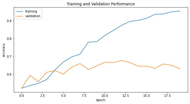
Let’s plot the history of the accuracy on both the training and validation sets.

history_plot()

• The model1 consistently achieves at least 52% validation accuracy in all 20 epochs. Furthermore, the accuracy of model1 stabilized between 60% and 67% during training.

• Compared to our baseline of 50% accuracy, model1 has approximately 10% - 17% more accuracy than the baseline.

• We can observe overfitting in the model1 because the training score is much higher than the validation score.

§3. Model with Data Augmentation

This section will improve our model performance by adding some data augmentation layers to our model. Data augmentation can increase the size of our training dataset to enhance performance. For example, a dog’s picture is still a picture of a dog even if we flip or shift the image horizontal and vertical, rotate the image to a different degree, and change the image’s brightness.

Before we create any data augmentation layers, let’s make a function called show_image_aumentation() to make a plot of the original image and a few copies to which data augmentation has been applied.

def show_image_aumentation (data_augmentation):
  """
  This function makes a plot of the original image 
  and a few copies to which data augmentation has been applied.
  """

  for images, labels in train_dataset.take(1):
    plt.figure(figsize=(10, 10))
    first_image = images[0]

    ax = plt.subplot(3, 3, 2)
    plt.imshow(first_image / 255)
    plt.title("original image")
    plt.axis('off')

    for i in range(6):
      ax = plt.subplot(3, 3, i + 4)
      augmented_image = data_augmentation(tf.expand_dims(first_image, 0))
      plt.imshow(augmented_image[0] / 255)
      plt.title("modified copies")
      plt.axis('off')

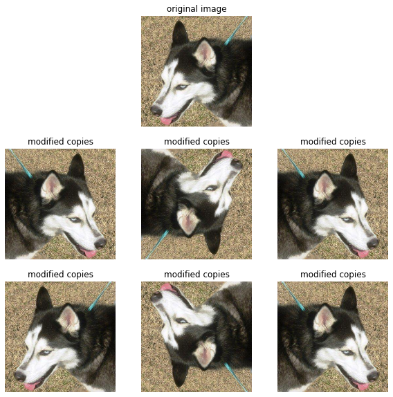
First, we will create a tf.keras.layers.RandomFlip() layer. This RandomFlip layer is a preprocessing layer that randomly flips images horizontally and/or vertically during training.

the attributes mode can be “horizontal”, “vertical”, or “horizontal_and_vertical”. Defaults to “horizontal_and_vertical”. “horizontal” is a left-right flip and “vertical” is a top-bottom flip.

random_flip_layer = tf.keras.Sequential(
    [
        tf.keras.layers.RandomFlip(mode = "horizontal_and_vertical"),

    ]
)

Let’s check our randomly flipped images.

show_image_aumentation(random_flip_layer)

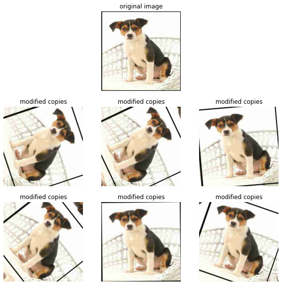
Next, we will create a tf.keras.layers.RandomRotation(). This RandomRotation layer is a preprocessing layer that randomly rotates images during training.

• factor=(-0.2, 0.3) results in an output rotation by a random amount in the range [-20% * 2pi, 30% * 2pi].
• factor=0.2 results in an output rotating by a random amount in the range [-20% * 2pi, 20% * 2pi].

random_rotation_layer = tf.keras.Sequential(
    [
        tf.keras.layers.RandomRotation(factor = 0.2),

    ]
)

Let’s check our randomly rotated images.

show_image_aumentation(random_rotation_layer)

Now, we have created two augmentation layers; let’s use these two augmentation layers in another tf.keras.models.Sequential model called model2, which is an improved version of model1.

model2 = tf.keras.Sequential([
      # augmentation layers                             
      tf.keras.layers.RandomFlip('horizontal'),
      # augmentation layers
      tf.keras.layers.RandomRotation(0.2),
      
      tf.keras.layers.Conv2D(32, (3, 3), activation='relu', input_shape=(160, 160, 3)),
      tf.keras.layers.MaxPooling2D((2, 2)),
      tf.keras.layers.Conv2D(32, (3, 3), activation='relu'),
      tf.keras.layers.MaxPooling2D((2, 2)),
      tf.keras.layers.Conv2D(64, (3, 3), activation='relu'),
      tf.keras.layers.MaxPooling2D((2, 2)),
      tf.keras.layers.Dropout(0.2),
      tf.keras.layers.Conv2D(64, (3, 3), activation='relu'),
      tf.keras.layers.MaxPooling2D((2, 2)),
      tf.keras.layers.Flatten(),
      tf.keras.layers.Dense(128, activation='relu'),
      tf.keras.layers.Dropout(0.2),
      tf.keras.layers.Dense(2, activation="softmax") # number of classes
     
])

model2.compile(optimizer="adam",
              loss=tf.keras.losses.SparseCategoricalCrossentropy(),
              metrics=['accuracy'])

history = model2.fit(train_dataset,
                    epochs=20, 
                    validation_data=validation_dataset)

I will show the last training epoch here:

Epoch 20/20
63/63 [==============================] - 7s 98ms/step - loss: 0.5798 - accuracy: 0.7075 - val_loss: 0.5827 - val_accuracy: 0.6980

    Epoch 1/20
    63/63 [==============================] - 6s 70ms/step - loss: 2.0127 - accuracy: 0.5140 - val_loss: 0.6862 - val_accuracy: 0.5384
    Epoch 2/20
    63/63 [==============================] - 4s 67ms/step - loss: 0.6902 - accuracy: 0.5375 - val_loss: 0.6907 - val_accuracy: 0.5371
    Epoch 3/20
    63/63 [==============================] - 5s 69ms/step - loss: 0.7059 - accuracy: 0.5440 - val_loss: 0.6879 - val_accuracy: 0.5557
    Epoch 4/20
    63/63 [==============================] - 5s 77ms/step - loss: 0.6881 - accuracy: 0.5485 - val_loss: 0.6512 - val_accuracy: 0.6089
    Epoch 5/20
    63/63 [==============================] - 6s 88ms/step - loss: 0.6751 - accuracy: 0.5925 - val_loss: 0.6489 - val_accuracy: 0.6300
    Epoch 6/20
    63/63 [==============================] - 8s 117ms/step - loss: 0.6553 - accuracy: 0.6155 - val_loss: 0.6258 - val_accuracy: 0.6609
    Epoch 7/20
    63/63 [==============================] - 8s 116ms/step - loss: 0.6437 - accuracy: 0.6290 - val_loss: 0.6389 - val_accuracy: 0.6176
    Epoch 8/20
    63/63 [==============================] - 7s 108ms/step - loss: 0.6206 - accuracy: 0.6585 - val_loss: 0.6165 - val_accuracy: 0.6708
    Epoch 9/20
    63/63 [==============================] - 7s 110ms/step - loss: 0.6244 - accuracy: 0.6570 - val_loss: 0.6135 - val_accuracy: 0.6832
    Epoch 10/20
    63/63 [==============================] - 4s 66ms/step - loss: 0.6265 - accuracy: 0.6645 - val_loss: 0.6149 - val_accuracy: 0.6646
    Epoch 11/20
    63/63 [==============================] - 4s 67ms/step - loss: 0.6113 - accuracy: 0.6615 - val_loss: 0.6188 - val_accuracy: 0.6349
    Epoch 12/20
    63/63 [==============================] - 4s 67ms/step - loss: 0.5955 - accuracy: 0.6825 - val_loss: 0.6071 - val_accuracy: 0.7067
    Epoch 13/20
    63/63 [==============================] - 4s 65ms/step - loss: 0.5976 - accuracy: 0.6835 - val_loss: 0.6066 - val_accuracy: 0.6807
    Epoch 14/20
    63/63 [==============================] - 4s 67ms/step - loss: 0.6030 - accuracy: 0.6700 - val_loss: 0.5908 - val_accuracy: 0.6968
    Epoch 15/20
    63/63 [==============================] - 5s 70ms/step - loss: 0.6243 - accuracy: 0.6545 - val_loss: 0.5757 - val_accuracy: 0.7104
    Epoch 16/20
    63/63 [==============================] - 5s 68ms/step - loss: 0.5749 - accuracy: 0.6950 - val_loss: 0.6180 - val_accuracy: 0.6584
    Epoch 17/20
    63/63 [==============================] - 5s 69ms/step - loss: 0.5819 - accuracy: 0.6905 - val_loss: 0.5608 - val_accuracy: 0.7203
    Epoch 18/20
    63/63 [==============================] - 5s 70ms/step - loss: 0.5904 - accuracy: 0.6910 - val_loss: 0.5675 - val_accuracy: 0.7030
    Epoch 19/20
    63/63 [==============================] - 7s 106ms/step - loss: 0.5810 - accuracy: 0.6900 - val_loss: 0.5596 - val_accuracy: 0.7215
    Epoch 20/20
    63/63 [==============================] - 7s 98ms/step - loss: 0.5798 - accuracy: 0.7075 - val_loss: 0.5827 - val_accuracy: 0.6980

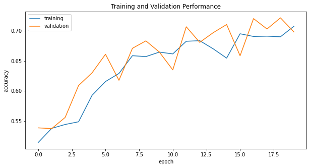
history_plot()

• The model2 consistently achieves at least 55% validation accuracy after epoch 3. Furthermore, the accuracy of model2 stabilized between 63% and 72% during training.

• We have a little bit higher validation accuracy than model1.

• However, our training and validating scores are much closer now, so I do not think model2 has a significant overfitting problem.

§4. Data Preprocessing

The image data has pixels with RGB values in the [0, 255] range. We should normalize the pixel value in the [0, 1] range or [-1, 1] range. Normalization images can increase the performance in many neural network models.

But if we handle the scaling prior to the training process, we can spend more of our training energy handling actual signal in the data and less energy having the weights adjust to the data scale.

The following code will create a preprocessing layer called preprocessor which we can slot into our model pipeline.

We used tf.keras.applications.mobilenet_v2.preprocess_input() which scales the input pixel in the [-1, 1] range.

i = tf.keras.Input(shape=(160, 160, 3))
x = tf.keras.applications.mobilenet_v2.preprocess_input(i)
preprocessor = tf.keras.Model(inputs = [i], outputs = [x])

Let’s incorporate the preprocessor layer inside another tf.keras.models.Sequential model called model3. The model3 is the improved version of the model2.

model3 = tf.keras.Sequential([
      preprocessor,
      # augmentation layers 
      tf.keras.layers.RandomFlip("horizontal"),
      # augmentation layers 
      tf.keras.layers.RandomRotation(0.2),

      tf.keras.layers.Conv2D(32, (3, 3), activation='relu', input_shape=(160, 160, 3)),
      tf.keras.layers.MaxPooling2D((2, 2)),
      tf.keras.layers.Conv2D(32, (3, 3), activation='relu'),
      tf.keras.layers.MaxPooling2D((2, 2)),
      tf.keras.layers.Conv2D(64, (3, 3), activation='relu'),
      tf.keras.layers.MaxPooling2D((2, 2)),
      tf.keras.layers.Dropout(0.2),
      tf.keras.layers.Conv2D(64, (3, 3), activation='relu'),
      tf.keras.layers.MaxPooling2D((2, 2)),
      tf.keras.layers.Flatten(),
      tf.keras.layers.Dense(128, activation='relu'),
      tf.keras.layers.Dropout(0.2),
      tf.keras.layers.Dense(2, activation="softmax") # number of classes
     
])

model3.compile(optimizer="adam",
              loss=tf.keras.losses.SparseCategoricalCrossentropy(),
              metrics=['accuracy'])

history = model3.fit(train_dataset,
                    epochs=20, 
                    validation_data=validation_dataset)

I will show the last training epoch here:

Epoch 20/20
63/63 [==============================] - 6s 94ms/step - loss: 0.4232 - accuracy: 0.7990 - val_loss: 0.4688 - val_accuracy: 0.7673

    Epoch 1/20
    63/63 [==============================] - 17s 86ms/step - loss: 0.6940 - accuracy: 0.5235 - val_loss: 0.6796 - val_accuracy: 0.5149
    Epoch 2/20
    63/63 [==============================] - 7s 103ms/step - loss: 0.6757 - accuracy: 0.5800 - val_loss: 0.6724 - val_accuracy: 0.5755
    Epoch 3/20
    63/63 [==============================] - 4s 62ms/step - loss: 0.6525 - accuracy: 0.6010 - val_loss: 0.6058 - val_accuracy: 0.6869
    Epoch 4/20
    63/63 [==============================] - 4s 62ms/step - loss: 0.6178 - accuracy: 0.6625 - val_loss: 0.5697 - val_accuracy: 0.7104
    Epoch 5/20
    63/63 [==============================] - 4s 61ms/step - loss: 0.5930 - accuracy: 0.6760 - val_loss: 0.5638 - val_accuracy: 0.7215
    Epoch 6/20
    63/63 [==============================] - 6s 93ms/step - loss: 0.5706 - accuracy: 0.7035 - val_loss: 0.5495 - val_accuracy: 0.7302
    Epoch 7/20
    63/63 [==============================] - 6s 87ms/step - loss: 0.5625 - accuracy: 0.7075 - val_loss: 0.5581 - val_accuracy: 0.7079
    Epoch 8/20
    63/63 [==============================] - 6s 90ms/step - loss: 0.5528 - accuracy: 0.7205 - val_loss: 0.5319 - val_accuracy: 0.7463
    Epoch 9/20
    63/63 [==============================] - 6s 92ms/step - loss: 0.5371 - accuracy: 0.7365 - val_loss: 0.5640 - val_accuracy: 0.7463
    Epoch 10/20
    63/63 [==============================] - 7s 97ms/step - loss: 0.5321 - accuracy: 0.7355 - val_loss: 0.5580 - val_accuracy: 0.7290
    Epoch 11/20
    63/63 [==============================] - 6s 95ms/step - loss: 0.5142 - accuracy: 0.7455 - val_loss: 0.5051 - val_accuracy: 0.7649
    Epoch 12/20
    63/63 [==============================] - 7s 111ms/step - loss: 0.5072 - accuracy: 0.7520 - val_loss: 0.5208 - val_accuracy: 0.7599
    Epoch 13/20
    63/63 [==============================] - 6s 83ms/step - loss: 0.5054 - accuracy: 0.7540 - val_loss: 0.4766 - val_accuracy: 0.7797
    Epoch 14/20
    63/63 [==============================] - 8s 115ms/step - loss: 0.4957 - accuracy: 0.7630 - val_loss: 0.5369 - val_accuracy: 0.7488
    Epoch 15/20
    63/63 [==============================] - 7s 102ms/step - loss: 0.4841 - accuracy: 0.7625 - val_loss: 0.4924 - val_accuracy: 0.7772
    Epoch 16/20
    63/63 [==============================] - 7s 108ms/step - loss: 0.4767 - accuracy: 0.7685 - val_loss: 0.4885 - val_accuracy: 0.7636
    Epoch 17/20
    63/63 [==============================] - 7s 96ms/step - loss: 0.4649 - accuracy: 0.7765 - val_loss: 0.4872 - val_accuracy: 0.7847
    Epoch 18/20
    63/63 [==============================] - 6s 88ms/step - loss: 0.4685 - accuracy: 0.7830 - val_loss: 0.4699 - val_accuracy: 0.7859
    Epoch 19/20
    63/63 [==============================] - 7s 108ms/step - loss: 0.4480 - accuracy: 0.7945 - val_loss: 0.4385 - val_accuracy: 0.8069
    Epoch 20/20
    63/63 [==============================] - 6s 94ms/step - loss: 0.4232 - accuracy: 0.7990 - val_loss: 0.4688 - val_accuracy: 0.7673

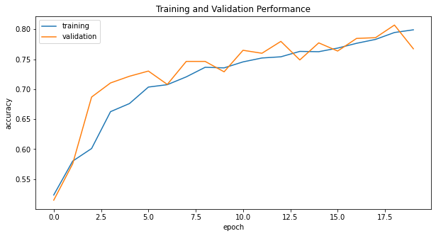
history_plot()

• The model3 consistently achieves at least 70% validation accuracy after epoch 4. Furthermore, the accuracy of model3 stabilized between 70% and 80% during training.

• The validation accuracy of model3 is much better than model2 and model1. Also, more than half of the validation accuracy at each epoch from model3 is higher than the highest score in model2.

• The training and validating scores are similar, so I do not observe a high chance of overfitting in the model3.

§5. Transfer Learning

In this section, we will explore transfer learning from a pre-trained model. The pre-trained model was previously trained on a large dataset. Therefore, we might find some pre-trained model that does the similary task we want to solve. Using a pre-trained model can save us some time without starting from scratch by training a large model on a large dataset.

We will create the base model from the MobileNetV2 model, which is pre-trained on the massive images data called ImageNet that contains more than 20000 classes. ImageNet provides a large image training dataset for research. Moreover, the dataset comprises various categories like fruit, cat, dog, etc. So, we can use this pre-trained model to help achieve our task here.

To do this, we need to first access a pre-existing “base model”, incorporate it into a full model for our current task, and then train that model.

The following code will download MobileNetV2 and configure it as a layer that can be included our your model.

IMG_SHAPE = IMG_SIZE + (3,)
base_model = tf.keras.applications.MobileNetV2(input_shape=IMG_SHAPE,
                                               include_top=False,
                                               weights='imagenet')
base_model.trainable = False

i = tf.keras.Input(shape=IMG_SHAPE)
x = base_model(i, training = False)
base_model_layer = tf.keras.Model(inputs = [i], outputs = [x])

Downloading data from https://storage.googleapis.com/tensorflow/keras-applications/mobilenet_v2/mobilenet_v2_weights_tf_dim_ordering_tf_kernels_1.0_160_no_top.h5
9412608/9406464 [==============================] - 0s 0us/step
9420800/9406464 [==============================] - 0s 0us/step

Let’s make another tf.keras.models.Sequential model called model4, which includes the pre-trained model.

model4 = tf.keras.Sequential([
      # the preprocessor layer from Part 4.                        
      preprocessor,
      # augmentation layers 
      tf.keras.layers.RandomFlip("horizontal"),
      # augmentation layers 
      tf.keras.layers.RandomRotation(0.2),
      # The base model layer constructed above
      base_model_layer,
      # additional layer
      tf.keras.layers.GlobalAveragePooling2D(),
      # additional layers
      tf.keras.layers.Dropout(0.2),
      # A Dense(2) layer at the very end to actually perform the classification.
      tf.keras.layers.Dense(2, activation="softmax") # number of classes
     
])

After we build the model, we can use the model.summary() method to display the overall contents from our model.

model4.summary()

Model: "sequential_9"
_________________________________________________________________
 Layer (type)                Output Shape              Param #   
=================================================================
 model (Functional)          (None, 160, 160, 3)       0         
                                                                 
 random_flip_8 (RandomFlip)  (None, 160, 160, 3)       0         
                                                                 
 random_rotation_6 (RandomRo  (None, 160, 160, 3)      0         
 tation)                                                         
                                                                 
 model_1 (Functional)        (None, 5, 5, 1280)        2257984   
                                                                 
 global_average_pooling2d (G  (None, 1280)             0         
 lobalAveragePooling2D)                                          
                                                                 
 dropout_10 (Dropout)        (None, 1280)              0         
                                                                 
 dense_10 (Dense)            (None, 2)                 2562      
                                                                 
=================================================================
Total params: 2,260,546
Trainable params: 2,562
Non-trainable params: 2,257,984
_________________________________________________________________

From the summary above, we notice that there are 2562 parameters to train in the model4, which is a lot! Also, there is a total of over 2.2 million parameters!

Then we can compile and train our model.

model4.compile(optimizer="adam",
              loss=tf.keras.losses.SparseCategoricalCrossentropy(),
              metrics=['accuracy'])

history = model4.fit(train_dataset,
                    epochs=20, 
                    validation_data=validation_dataset)

I will show the last training epoch here:

Epoch 20/20
63/63 [==============================] - 7s 101ms/step - loss: 0.1028 - accuracy: 0.9620 - val_loss: 0.0485 - val_accuracy: 0.9839

    Epoch 1/20
    63/63 [==============================] - 9s 91ms/step - loss: 0.2822 - accuracy: 0.8765 - val_loss: 0.0739 - val_accuracy: 0.9765
    Epoch 2/20
    63/63 [==============================] - 5s 70ms/step - loss: 0.1433 - accuracy: 0.9360 - val_loss: 0.0580 - val_accuracy: 0.9827
    Epoch 3/20
    63/63 [==============================] - 5s 70ms/step - loss: 0.1435 - accuracy: 0.9440 - val_loss: 0.0510 - val_accuracy: 0.9814
    Epoch 4/20
    63/63 [==============================] - 5s 71ms/step - loss: 0.1307 - accuracy: 0.9500 - val_loss: 0.0576 - val_accuracy: 0.9777
    Epoch 5/20
    63/63 [==============================] - 5s 70ms/step - loss: 0.1205 - accuracy: 0.9525 - val_loss: 0.0459 - val_accuracy: 0.9839
    Epoch 6/20
    63/63 [==============================] - 5s 70ms/step - loss: 0.1114 - accuracy: 0.9565 - val_loss: 0.0400 - val_accuracy: 0.9876
    Epoch 7/20
    63/63 [==============================] - 5s 70ms/step - loss: 0.1121 - accuracy: 0.9500 - val_loss: 0.0433 - val_accuracy: 0.9864
    Epoch 8/20
    63/63 [==============================] - 5s 70ms/step - loss: 0.1220 - accuracy: 0.9510 - val_loss: 0.0474 - val_accuracy: 0.9851
    Epoch 9/20
    63/63 [==============================] - 5s 80ms/step - loss: 0.1211 - accuracy: 0.9530 - val_loss: 0.0503 - val_accuracy: 0.9802
    Epoch 10/20
    63/63 [==============================] - 5s 76ms/step - loss: 0.1138 - accuracy: 0.9550 - val_loss: 0.0615 - val_accuracy: 0.9765
    Epoch 11/20
    63/63 [==============================] - 5s 71ms/step - loss: 0.0938 - accuracy: 0.9615 - val_loss: 0.0512 - val_accuracy: 0.9802
    Epoch 12/20
    63/63 [==============================] - 5s 70ms/step - loss: 0.0980 - accuracy: 0.9610 - val_loss: 0.0386 - val_accuracy: 0.9839
    Epoch 13/20
    63/63 [==============================] - 6s 97ms/step - loss: 0.0883 - accuracy: 0.9650 - val_loss: 0.0450 - val_accuracy: 0.9814
    Epoch 14/20
    63/63 [==============================] - 8s 124ms/step - loss: 0.1014 - accuracy: 0.9605 - val_loss: 0.0455 - val_accuracy: 0.9839
    Epoch 15/20
    63/63 [==============================] - 5s 70ms/step - loss: 0.0895 - accuracy: 0.9645 - val_loss: 0.0350 - val_accuracy: 0.9864
    Epoch 16/20
    63/63 [==============================] - 8s 116ms/step - loss: 0.0969 - accuracy: 0.9590 - val_loss: 0.0471 - val_accuracy: 0.9827
    Epoch 17/20
    63/63 [==============================] - 7s 107ms/step - loss: 0.0903 - accuracy: 0.9640 - val_loss: 0.0397 - val_accuracy: 0.9864
    Epoch 18/20
    63/63 [==============================] - 5s 69ms/step - loss: 0.0857 - accuracy: 0.9625 - val_loss: 0.0494 - val_accuracy: 0.9827
    Epoch 19/20
    63/63 [==============================] - 6s 86ms/step - loss: 0.0964 - accuracy: 0.9600 - val_loss: 0.0424 - val_accuracy: 0.9839
    Epoch 20/20
    63/63 [==============================] - 7s 101ms/step - loss: 0.1028 - accuracy: 0.9620 - val_loss: 0.0485 - val_accuracy: 0.9839

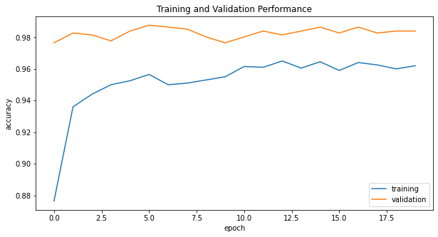
history_plot()

• The model4 consistently achieves at least 95% validation accuracy at every epoch. Furthermore, the accuracy of model4 stabilized between 97% and 99% during training.

• The validation accuracy of model4 is outstanding; it’s the best model in this post.

• The validation accuracy of model4 is higher than the training accuracy; I don’t think model4 is overfitting.

§6. Score on Test Data

Let’s evaluate our model’s perforance from test dataset.

model4.evaluate(test_dataset)

6/6 [==============================] - 1s 84ms/step - loss: 0.0719 - accuracy: 0.9792

[0.07189350575208664, 0.9791666865348816]

Using the pre-trained model, which correctly predicts the cat or dog images with approximately 98% accuracy, that’s pretty impressive.