Blog Post 6 - Fake News Classification

In this Blog Post, we will use TensorFlow techniques to find out if any articles contain fake news.

Acknowledgment

Major parts of this Blog Post assignment, including several code chunks and explanations, are based on Professor Phil Chodrow.

Let’s put all import statements here at the beginning for convenience.

import pandas as pd
import string
import numpy as np
import re
import tensorflow as tf
from matplotlib import pyplot as plt
from tensorflow import keras
from tensorflow.keras import layers
from tensorflow.keras import losses
from tensorflow.keras.layers.experimental.preprocessing import TextVectorization

# for embedding viz
import plotly.express as px 
import plotly.io as pio
pio.templates.default = "plotly_white"

import nltk
nltk.download('stopwords')
from nltk.corpus import stopwords

[nltk_data] Downloading package stopwords to /root/nltk_data...
[nltk_data]   Package stopwords is already up-to-date!

§1. Acquire Training Data

In this section, we will download the data from the article

Ahmed H, Traore I, Saad S. (2017) “Detection of Online Fake News Using N-Gram Analysis and Machine Learning Techniques. In: Traore I., Woungang I., Awad A. (eds) Intelligent, Secure, and Dependable Systems in Distributed and Cloud Environments. ISDDC 2017. Lecture Notes in Computer Science, vol 10618. Springer, Cham (pp. 127-138).

Once we have load the articles into a pandas dataframe, we can take a look at the first five rows of the dataset using df.head().

train_url = "https://github.com/PhilChodrow/PIC16b/blob/master/datasets/fake_news_train.csv?raw=true"
df = pd.read_csv(train_url)
df.head()

	Unnamed: 0	title	text	fake
0	17366	Merkel: Strong result for Austria's FPO 'big c...	German Chancellor Angela Merkel said on Monday...	0
1	5634	Trump says Pence will lead voter fraud panel	WEST PALM BEACH, Fla.President Donald Trump sa...	0
2	17487	JUST IN: SUSPECTED LEAKER and “Close Confidant...	On December 5, 2017, Circa s Sara Carter warne...	1
3	12217	Thyssenkrupp has offered help to Argentina ove...	Germany s Thyssenkrupp, has offered assistance...	0
4	5535	Trump say appeals court decision on travel ban...	President Donald Trump on Thursday called the ...	0

The data set contains four columns, each row of the data corresponds to an article, and some important column heading variables have the following meanings:

title : The title of the article
text : The full article text
fake : 0 if the article is true; 1 if the article contains fake news

Next, we will use df.isna() to pick out all nan values from data, then use df.sum() to find how many nan values are in each column and save the result in nan_values_summary.

nan_values_summary = df.isna().sum()
nan_values_summary

Unnamed: 0    0
title         0
text          0
fake          0
dtype: int64

Wow, it looks like we don’t have any missing values, which is good.

Next, let’s make a bar chart to visualize the distribution of fake articles

import seaborn as sns
x = df.groupby("fake").apply(len)
fig, ax = plt.subplots(1)
ax = sns.barplot(x =x.index,y=x.values )
ax.set(title = "Bar Charts of Fake News")
# remove border
ax.spines['right'].set_visible(False)
ax.spines['top'].set_visible(False)

# I find how to add annotate on each bar online from 
# https://www.geeksforgeeks.org/how-to-annotate-bars-in-barplot-with-matplotlib-in-python/
# Iterrating over the bars one-by-one
for bar in ax.patches: 
  # Using Matplotlib's annotate function and
  # passing the coordinates where the annotation shall be done
  # x-coordinate: bar.get_x() + bar.get_width() / 2
  # y-coordinate: bar.get_height()
  # free space to be left to make graph pleasing: (0, 8)
  # ha and va stand for the horizontal and vertical alignment
  ax.annotate(int(bar.get_height()),
             (bar.get_x() + bar.get_width() / 2 , bar.get_height()),
              ha='center', va='center', size=10, xytext=(0, 6),
              textcoords='offset points', color="firebrick") 

blog post 6 bar charts

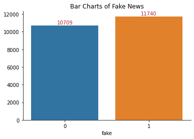
The number of articles that are fake or not is approximately similar.

§2. Make a Dataset

In this section, we change our data frame into a TensorFlow Dataset. We will use tf.data.Dataset.from_tensor_slices(),to make our dataset.

After successfully creating the Dataset, we need to do data cleaning. For instance, we should remove stopwords from the articles. The stopwords are usually considered as useless information; such as commonly used words (“the,” “and,” “but,” “a”, “an”, or “in”)

Luckily, we don’t have to create the list of stopwords by ourselves. Instead, we can use the natural language toolkit (NLTK) to get all stopwords we need from the package nltk.corpus. Here are some examples of how to use nltk.

First, let’s create a function called make_dataset(), which has the following property:

Removing stopwords from the article text and title
Constructing and returning a tf.data.Dataset with two inputs (title, text) and one output (fake). Because we have multiple inputs, we are going to construct our Dataset from a tuple of dictionaries. The first dictionary is going to specify the different components in the predictor data (title, text), while the second dictionary is going to specify the different components of the target data (fake).

def make_dataset(panda_df):
  """
  This function will remove stopwords from the article text and title
  in the training data frame,then create a TensorFlow Dataset from the
  cleaned training data frame.

  Parameters
  ----------
  panda_df: data frame; 

  Return 
  ----------
  tf_dataset: TensorFlow Dataset; 
  """

  # get stopwords from 'nltk.corpus' package
  stop = stopwords.words('english')

  # removing stopwords from the article text and title
  panda_df[['title','text']].apply(lambda x: [item for item in x if item not in stop])

  # Construct and return a tf.data.Dataset with two inputs (title, text) and one output (fake)
  tf_dataset = tf.data.Dataset.from_tensor_slices(
        (
            {
                "title" : df[["title"]],
                "text"  : df["text"]
            },
            {
                "fake" : df[["fake"]] # second dictionary
            }
        )
     )
  
  # batch our Dataset prior to returning it
  tf_dataset = tf_dataset.batch(100)
  return tf_dataset

The tf_dataset.batch(100) will process 100 pieces of data at a time when doing stochastic gradient descent. Using batch can faster the training process, but it will decrease the accuracy.

Now, let’s use our function make_dataaset() to create the dataset.

data = make_dataset(panda_df=df)

Validation Data

This section will perform a train and validation split on our dataset. We will split 20% of the training dataset as validation.

We can create a function called split_dataset() to perform a train and validation split.

def split_dataset(data, train_size):
  """
  This function will perform a train and validation split on input dataset

  Parameters
  ----------
  data: dataset; 
  train_size: float (0.0 - 1.0); size of the training dataset.

  Return 
  ----------
  train: training dataset
  val: validation dataset
  """

  # randomly shuffle the data
  data = data.shuffle(buffer_size = len(data))
  # size of the training data
  train_size = int(0.8*len(data))
  # 80% data as the training data
  train = data.take(train_size)
  # 20% data as the validation data
  val  = data.skip(train_size)
  
  return train, val

Let’s use the function split_dataset() to spilt our data.

train_dataset, val_dataset = split_dataset(data, train_size=0.8)

Let’s check the length of our training and validation dataset.

len(train_dataset), len(val_dataset)

(180, 45)

We have 180 and 45 batches of data in our training and validation dataset. We used the batched size of 100 when creating our Dataset, so we should multiply by the batch size 100 to get the total number of rows in each Dataset.

Base Rate

Here we will calculate the base rate of our mode. Base rate refers to the accuracy of a model that always makes the same guess (for example, such a model might always say “fake news!”).

The following line of code will create an iterator called labels for the train_dataset.

labels_iterator= train_dataset.unbatch().map(lambda x, label: label['fake'][0]).as_numpy_iterator()

Next, we will caculate total number of articles and how many are labels as fake in our training datase.

label 0 : The article is true
label 1 : The article contains fake news

train_labels_list =list(labels_iterator)
num_labels = len(train_labels_list)
num_fake  = train_labels_list.count(0)
print("Totoal number of labels " + str(num_labels))
print("Total number of fake: " + str(num_fake))
print("Base Rate \u2248 " + str(round(num_fake/num_labels *100, 4)) + "%")

Totoal number of labels 17949
Total number of fake: 8544
Base Rate ≈ 47.6015%

§3. Create Models

This section will create three different TensorFlow models to determine the effective way of detecting fake news.

First, we will focus on only the title of the article.
Second, we will focus on only the text of the article.
Third, we will focus on both title and text of the article.

Preprocessing

Before building our model, we should do text preprocessing on our dataset.

Standardization

Standardization refers to the act of taking a some text that’s “messy” in some way and making it less messy. Common standardizations include:

Removing capitals.
Removing punctuation.
Removing HTML elements or other non-semantic content.

We will standardize the text date into lowercase and remove all punctuations in the next cell.

def standardization(input_data):
    lowercase = tf.strings.lower(input_data)
    no_punctuation = tf.strings.regex_replace(lowercase,
                                  '[%s]' % re.escape(string.punctuation),'')
    return no_punctuation 

Vectorization

Text Vectorization refers to the process of representing text as a vector (array, tensor).

Here, we’ll replace each word by its frequency rank in the data.

the text layer will help us turn our text information ( title, text) into numbers by replacing each word with its rank frequency in the data

# only the top 2600 distinct words will be tracked
size_vocabulary = 2600

vectorize_layer = TextVectorization(
    standardize=standardization,
    max_tokens=size_vocabulary, # only consider this many words
    output_mode='int',
    output_sequence_length=500) 

We need to adapt the vectorization layer to the title and text. In the adaptation process, the vectorization layer learns what words are common in the title and text.

vectorize_layer.adapt(train_dataset.map(lambda x, y: x["title"]))
vectorize_layer.adapt(train_dataset.map(lambda x, y: x["text"]))

Inputs

We need to create two ‘keras.Input’ for title and text for our model. The title column contains just one article title, and the text column contains just one full article text, so both inputs have a shape (1, ). The name should match when we constructed the dataset using tf.data.Dataset.from_tensor_slices() early. Since both inputs contain text, we should set the type as a string.

title_input = keras.Input(
    shape = (1,), 
    name = "title",
    dtype = "string"
)

text_input = keras.Input(
    shape = (1,), 
    name = "text",
    dtype = "string"
)

Shared Layers

When using functional API, we might use the same layer in the model. Shared Layers are same layers which we used mutiple time in different part of the model. We will make an Embedding layer which is shared with title_input and text_input.

# Embedding for 2600 unique words mapped to 3-dimentional vectors
shared_embedding = layers.Embedding(size_vocabulary, output_dim = 3, name = "embedding" )

First Model

We will only use the article title as input in the first model.

Let’s write the pipeline for the title.

# pipeline for the first model only focuses on the title

title_features = vectorize_layer(title_input)
# Reuse the same Embedding layer to encode title inputs
title_features = shared_embedding(title_features)
# add Droupout layer to reduce overfitting
title_features = layers.Dropout(0.2)(title_features)
# GlobalAveragePooling1D similar to MaxPooling layer
title_features = layers.GlobalAveragePooling1D()(title_features)
# add Droupout layer to reduce overfitting
title_features = layers.Dropout(0.2)(title_features)
title_features = layers.Dense(32, activation='relu')(title_features)
title_features = layers.Dropout(0.2)(title_features)
# each data point (title) will be represented as 32 numbers
title_features = layers.Dense(32, activation='relu')(title_features)

We should give the output layer a name that matches the key corresponding to the target data in the Dataset we will pass to the model. In our case, the name should be ‘fake.’ This is how TensorFlow knows which part of our data set to compare against the outputs!

# output layer for the first model
title_output = layers.Dense(2, name = "fake")(title_features)

Then, we can create the first model.

title_model = keras.Model(
      inputs = title_input,
      outputs = title_output
)

complie the model

title_model.compile(optimizer = "adam",
                loss = losses.SparseCategoricalCrossentropy(from_logits=True),
                metrics=['accuracy']
)

train the model

title_history = title_model.fit(train_dataset, 
                                validation_data=val_dataset,
                                epochs = 30)

Click to show all 30 epochs from the first model.


    Epoch 1/30


    /usr/local/lib/python3.7/dist-packages/keras/engine/functional.py:559: UserWarning: Input dict contained keys ['text'] which did not match any model input. They will be ignored by the model.
      inputs = self._flatten_to_reference_inputs(inputs)


    180/180 [==============================] - 4s 11ms/step - loss: 0.6919 - accuracy: 0.5249 - val_loss: 0.6902 - val_accuracy: 0.5367
    Epoch 2/30
    180/180 [==============================] - 1s 7ms/step - loss: 0.6886 - accuracy: 0.5403 - val_loss: 0.6772 - val_accuracy: 0.5273
    Epoch 3/30
    180/180 [==============================] - 1s 5ms/step - loss: 0.5496 - accuracy: 0.7633 - val_loss: 0.3428 - val_accuracy: 0.8789
    Epoch 4/30
    180/180 [==============================] - 1s 5ms/step - loss: 0.3006 - accuracy: 0.8832 - val_loss: 0.2292 - val_accuracy: 0.9071
    Epoch 5/30
    180/180 [==============================] - 1s 5ms/step - loss: 0.2528 - accuracy: 0.8985 - val_loss: 0.1858 - val_accuracy: 0.9294
    Epoch 6/30
    180/180 [==============================] - 1s 5ms/step - loss: 0.2289 - accuracy: 0.9082 - val_loss: 0.1728 - val_accuracy: 0.9329
    Epoch 7/30
    180/180 [==============================] - 1s 5ms/step - loss: 0.2112 - accuracy: 0.9163 - val_loss: 0.1719 - val_accuracy: 0.9342
    Epoch 8/30
    180/180 [==============================] - 1s 5ms/step - loss: 0.2013 - accuracy: 0.9198 - val_loss: 0.1470 - val_accuracy: 0.9449
    Epoch 9/30
    180/180 [==============================] - 1s 5ms/step - loss: 0.1969 - accuracy: 0.9228 - val_loss: 0.1517 - val_accuracy: 0.9438
    Epoch 10/30
    180/180 [==============================] - 1s 5ms/step - loss: 0.1870 - accuracy: 0.9277 - val_loss: 0.1423 - val_accuracy: 0.9487
    Epoch 11/30
    180/180 [==============================] - 1s 6ms/step - loss: 0.1806 - accuracy: 0.9307 - val_loss: 0.1516 - val_accuracy: 0.9431
    Epoch 12/30
    180/180 [==============================] - 1s 5ms/step - loss: 0.1804 - accuracy: 0.9310 - val_loss: 0.1315 - val_accuracy: 0.9480
    Epoch 13/30
    180/180 [==============================] - 1s 6ms/step - loss: 0.1724 - accuracy: 0.9348 - val_loss: 0.1486 - val_accuracy: 0.9444
    Epoch 14/30
    180/180 [==============================] - 1s 5ms/step - loss: 0.1719 - accuracy: 0.9343 - val_loss: 0.1432 - val_accuracy: 0.9436
    Epoch 15/30
    180/180 [==============================] - 1s 5ms/step - loss: 0.1666 - accuracy: 0.9380 - val_loss: 0.1408 - val_accuracy: 0.9484
    Epoch 16/30
    180/180 [==============================] - 1s 5ms/step - loss: 0.1630 - accuracy: 0.9372 - val_loss: 0.1215 - val_accuracy: 0.9564
    Epoch 17/30
    180/180 [==============================] - 1s 5ms/step - loss: 0.1654 - accuracy: 0.9379 - val_loss: 0.1156 - val_accuracy: 0.9600
    Epoch 18/30
    180/180 [==============================] - 1s 5ms/step - loss: 0.1592 - accuracy: 0.9403 - val_loss: 0.1294 - val_accuracy: 0.9511
    Epoch 19/30
    180/180 [==============================] - 1s 5ms/step - loss: 0.1685 - accuracy: 0.9358 - val_loss: 0.1400 - val_accuracy: 0.9456
    Epoch 20/30
    180/180 [==============================] - 1s 6ms/step - loss: 0.1609 - accuracy: 0.9392 - val_loss: 0.1152 - val_accuracy: 0.9593
    Epoch 21/30
    180/180 [==============================] - 1s 5ms/step - loss: 0.1543 - accuracy: 0.9413 - val_loss: 0.1191 - val_accuracy: 0.9531
    Epoch 22/30
    180/180 [==============================] - 1s 5ms/step - loss: 0.1514 - accuracy: 0.9411 - val_loss: 0.1189 - val_accuracy: 0.9591
    Epoch 23/30
    180/180 [==============================] - 1s 5ms/step - loss: 0.1516 - accuracy: 0.9422 - val_loss: 0.1130 - val_accuracy: 0.9573
    Epoch 24/30
    180/180 [==============================] - 1s 5ms/step - loss: 0.1535 - accuracy: 0.9403 - val_loss: 0.1072 - val_accuracy: 0.9613
    Epoch 25/30
    180/180 [==============================] - 1s 5ms/step - loss: 0.1473 - accuracy: 0.9450 - val_loss: 0.0979 - val_accuracy: 0.9689
    Epoch 26/30
    180/180 [==============================] - 1s 5ms/step - loss: 0.1508 - accuracy: 0.9435 - val_loss: 0.0973 - val_accuracy: 0.9664
    Epoch 27/30
    180/180 [==============================] - 1s 5ms/step - loss: 0.1494 - accuracy: 0.9445 - val_loss: 0.1046 - val_accuracy: 0.9629
    Epoch 28/30
    180/180 [==============================] - 1s 5ms/step - loss: 0.1523 - accuracy: 0.9414 - val_loss: 0.1030 - val_accuracy: 0.9633
    Epoch 29/30
    180/180 [==============================] - 1s 5ms/step - loss: 0.1431 - accuracy: 0.9452 - val_loss: 0.1137 - val_accuracy: 0.9600
    Epoch 30/30
    180/180 [==============================] - 1s 6ms/step - loss: 0.1498 - accuracy: 0.9441 - val_loss: 0.1010 - val_accuracy: 0.9658

Next, we will create a function called history_plot(), which will plot the history of the accuracy on both the training and validation sets.

def history_plot(history, model_name):
  """
  This function will create the plot of accuracy on the training and validation sets

  Parameters
  ----------
  history: history object; it holds a record of the loss values and metric values during training
  model_name: string; The name for the model

  Return 
  ----------
  No return value 
  """
  fig, ax = plt.subplots(1,1, figsize=(10,5))
  ax.yaxis.set_major_locator(plt.MaxNLocator(10))
  plt.plot(history.history["accuracy"], label = "training")
  plt.plot(history.history["val_accuracy"], label = "validation")
  plt.gca().set(xlabel = "epoch", ylabel = "accuracy")
  plt.title("Training and Validation Performance of " + model_name)
  plt.legend()

Let’s plot the history of the accuracy on both the training and validation sets for the first model.

history_plot(title_history, model_name= "First Model")

blog post 6 model1 history

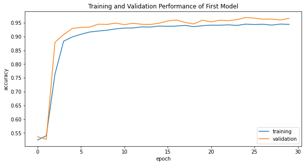
The first model consistently scores between 94% - 96% validation accuracy after epoch 8, which is acceptable.

Second Model

We will only use the article text as input in the second model.

Let’s write the pipeline for the text.

# pipeline for the second model only focuses on the text

text_features = vectorize_layer(text_input)
# Reuse the same Embedding layer to encode title inputs
text_features = shared_embedding(text_features)
# add Droupout layer to reduce overfitting
text_features = layers.Dropout(0.2)(text_features)
# GlobalAveragePooling1D similar to MaxPooling layer
text_features = layers.GlobalAveragePooling1D()(text_features)
# add Droupout layer to reduce overfitting
text_features = layers.Dropout(0.2)(text_features)
text_features = layers.Dense(32, activation='relu')(text_features)
text_features = layers.Dropout(0.2)(text_features)
# each data point (title) will be represented as 32 numbers
text_features = layers.Dense(32, activation='relu')(text_features)

# output layer for the second model
text_output = layers.Dense(2, name = "fake")(text_features)

Then, we can create, compile and train the second model.

text_model = keras.Model(
     inputs = [text_input],
     outputs = text_output
)

text_model.compile(optimizer = "adam",
                  loss = losses.SparseCategoricalCrossentropy(from_logits=True),
                  metrics=['accuracy']
)

text_history = text_model.fit(train_dataset, 
                              validation_data=val_dataset,
                              epochs = 30)

Click to show all 30 epochs from the second model.


    Epoch 1/30


    /usr/local/lib/python3.7/dist-packages/keras/engine/functional.py:559: UserWarning: Input dict contained keys ['title'] which did not match any model input. They will be ignored by the model.
      inputs = self._flatten_to_reference_inputs(inputs)


    180/180 [==============================] - 3s 14ms/step - loss: 0.6026 - accuracy: 0.6691 - val_loss: 0.4291 - val_accuracy: 0.8613
    Epoch 2/30
    180/180 [==============================] - 2s 13ms/step - loss: 0.3333 - accuracy: 0.8716 - val_loss: 0.2620 - val_accuracy: 0.8827
    Epoch 3/30
    180/180 [==============================] - 2s 13ms/step - loss: 0.2211 - accuracy: 0.9227 - val_loss: 0.2307 - val_accuracy: 0.8929
    Epoch 4/30
    180/180 [==============================] - 2s 13ms/step - loss: 0.1795 - accuracy: 0.9389 - val_loss: 0.2435 - val_accuracy: 0.8929
    Epoch 5/30
    180/180 [==============================] - 2s 13ms/step - loss: 0.1646 - accuracy: 0.9440 - val_loss: 0.2013 - val_accuracy: 0.9080
    Epoch 6/30
    180/180 [==============================] - 2s 13ms/step - loss: 0.1447 - accuracy: 0.9531 - val_loss: 0.1952 - val_accuracy: 0.9065
    Epoch 7/30
    180/180 [==============================] - 2s 13ms/step - loss: 0.1328 - accuracy: 0.9573 - val_loss: 0.1883 - val_accuracy: 0.9111
    Epoch 8/30
    180/180 [==============================] - 2s 13ms/step - loss: 0.1198 - accuracy: 0.9620 - val_loss: 0.1510 - val_accuracy: 0.9287
    Epoch 9/30
    180/180 [==============================] - 2s 13ms/step - loss: 0.1149 - accuracy: 0.9641 - val_loss: 0.1360 - val_accuracy: 0.9360
    Epoch 10/30
    180/180 [==============================] - 2s 13ms/step - loss: 0.1078 - accuracy: 0.9650 - val_loss: 0.1537 - val_accuracy: 0.9253
    Epoch 11/30
    180/180 [==============================] - 2s 13ms/step - loss: 0.0963 - accuracy: 0.9693 - val_loss: 0.1533 - val_accuracy: 0.9276
    Epoch 12/30
    180/180 [==============================] - 2s 13ms/step - loss: 0.0945 - accuracy: 0.9689 - val_loss: 0.1251 - val_accuracy: 0.9440
    Epoch 13/30
    180/180 [==============================] - 2s 13ms/step - loss: 0.0870 - accuracy: 0.9724 - val_loss: 0.1015 - val_accuracy: 0.9540
    Epoch 14/30
    180/180 [==============================] - 3s 14ms/step - loss: 0.0837 - accuracy: 0.9735 - val_loss: 0.1140 - val_accuracy: 0.9444
    Epoch 15/30
    180/180 [==============================] - 2s 13ms/step - loss: 0.0846 - accuracy: 0.9722 - val_loss: 0.0788 - val_accuracy: 0.9609
    Epoch 16/30
    180/180 [==============================] - 3s 17ms/step - loss: 0.0762 - accuracy: 0.9749 - val_loss: 0.1171 - val_accuracy: 0.9453
    Epoch 17/30
    180/180 [==============================] - 3s 17ms/step - loss: 0.0680 - accuracy: 0.9774 - val_loss: 0.0775 - val_accuracy: 0.9589
    Epoch 18/30
    180/180 [==============================] - 2s 13ms/step - loss: 0.0665 - accuracy: 0.9775 - val_loss: 0.1104 - val_accuracy: 0.9480
    Epoch 19/30
    180/180 [==============================] - 2s 13ms/step - loss: 0.0668 - accuracy: 0.9773 - val_loss: 0.0673 - val_accuracy: 0.9669
    Epoch 20/30
    180/180 [==============================] - 3s 14ms/step - loss: 0.0622 - accuracy: 0.9788 - val_loss: 0.0720 - val_accuracy: 0.9613
    Epoch 21/30
    180/180 [==============================] - 2s 13ms/step - loss: 0.0584 - accuracy: 0.9801 - val_loss: 0.0706 - val_accuracy: 0.9633
    Epoch 22/30
    180/180 [==============================] - 2s 13ms/step - loss: 0.0568 - accuracy: 0.9802 - val_loss: 0.0597 - val_accuracy: 0.9709
    Epoch 23/30
    180/180 [==============================] - 2s 13ms/step - loss: 0.0567 - accuracy: 0.9799 - val_loss: 0.0397 - val_accuracy: 0.9900
    Epoch 24/30
    180/180 [==============================] - 2s 13ms/step - loss: 0.0525 - accuracy: 0.9814 - val_loss: 0.0671 - val_accuracy: 0.9683
    Epoch 25/30
    180/180 [==============================] - 2s 13ms/step - loss: 0.0501 - accuracy: 0.9827 - val_loss: 0.0712 - val_accuracy: 0.9656
    Epoch 26/30
    180/180 [==============================] - 3s 15ms/step - loss: 0.0464 - accuracy: 0.9837 - val_loss: 0.0424 - val_accuracy: 0.9889
    Epoch 27/30
    180/180 [==============================] - 4s 22ms/step - loss: 0.0473 - accuracy: 0.9845 - val_loss: 0.0434 - val_accuracy: 0.9900
    Epoch 28/30
    180/180 [==============================] - 5s 27ms/step - loss: 0.0466 - accuracy: 0.9839 - val_loss: 0.0462 - val_accuracy: 0.9738
    Epoch 29/30
    180/180 [==============================] - 4s 24ms/step - loss: 0.0459 - accuracy: 0.9836 - val_loss: 0.0491 - val_accuracy: 0.9716
    Epoch 30/30
    180/180 [==============================] - 5s 27ms/step - loss: 0.0430 - accuracy: 0.9847 - val_loss: 0.0395 - val_accuracy: 0.9769

Let’s plot the history of the accuracy on both the training and validation sets for the second model.

history_plot(text_history, model_name="Second Model")

blog post 6 model2 history

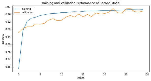
The second model consistently scores around 95% - 99% validation accuracy after half epochs (epoch 15), which is not bad.

Third Model

In the third model, we will use both the article title and the article text as input.

First, we should concatenate the output of the title pipeline and the output of the text pipeline.

main = layers.concatenate([title_features, text_features], axis=1)

Then, we add one more Dense layer for the third model.

main = layers.Dense(32, activation='relu')(main)
num_class = 2
# output layer for the third model
output = layers.Dense(num_class, name = "fake")(main)

Let’s create the model.

main_model = keras.Model(
    inputs = [title_input, text_input],
    outputs = output
)

Let’s check the third model’s structure by using the model.summary().

main_model.summary()

Model: "model_2"
__________________________________________________________________________________________________
 Layer (type)                   Output Shape         Param #     Connected to                     
==================================================================================================
 title (InputLayer)             [(None, 1)]          0           []                               
                                                                                                  
 text (InputLayer)              [(None, 1)]          0           []                               
                                                                                                  
 text_vectorization (TextVector  (None, 500)         0           ['title[0][0]',                  
 ization)                                                         'text[0][0]']                   
                                                                                                  
 embedding (Embedding)          (None, 500, 3)       7800        ['text_vectorization[0][0]',     
                                                                  'text_vectorization[1][0]']     
                                                                                                  
 dropout (Dropout)              (None, 500, 3)       0           ['embedding[0][0]']              
                                                                                                  
 dropout_3 (Dropout)            (None, 500, 3)       0           ['embedding[1][0]']              
                                                                                                  
 global_average_pooling1d (Glob  (None, 3)           0           ['dropout[0][0]']                
 alAveragePooling1D)                                                                              
                                                                                                  
 global_average_pooling1d_1 (Gl  (None, 3)           0           ['dropout_3[0][0]']              
 obalAveragePooling1D)                                                                            
                                                                                                  
 dropout_1 (Dropout)            (None, 3)            0           ['global_average_pooling1d[0][0]'
                                                                 ]                                
                                                                                                  
 dropout_4 (Dropout)            (None, 3)            0           ['global_average_pooling1d_1[0][0
                                                                 ]']                              
                                                                                                  
 dense (Dense)                  (None, 32)           128         ['dropout_1[0][0]']              
                                                                                                  
 dense_2 (Dense)                (None, 32)           128         ['dropout_4[0][0]']              
                                                                                                  
 dropout_2 (Dropout)            (None, 32)           0           ['dense[0][0]']                  
                                                                                                  
 dropout_5 (Dropout)            (None, 32)           0           ['dense_2[0][0]']                
                                                                                                  
 dense_1 (Dense)                (None, 32)           1056        ['dropout_2[0][0]']              
                                                                                                  
 dense_3 (Dense)                (None, 32)           1056        ['dropout_5[0][0]']              
                                                                                                  
 concatenate (Concatenate)      (None, 64)           0           ['dense_1[0][0]',                
                                                                  'dense_3[0][0]']                
                                                                                                  
 dense_4 (Dense)                (None, 32)           2080        ['concatenate[0][0]']            
                                                                                                  
 fake (Dense)                   (None, 2)            66          ['dense_4[0][0]']                
                                                                                                  
==================================================================================================
Total params: 12,314
Trainable params: 12,314
Non-trainable params: 0
__________________________________________________________________________________________________

The third model has over 12 thousand parameters.

We also can create a visual version of the structure for the third model by using the plot_model function.

keras.utils.plot_model(main_model)

blog post 6 model3 structure

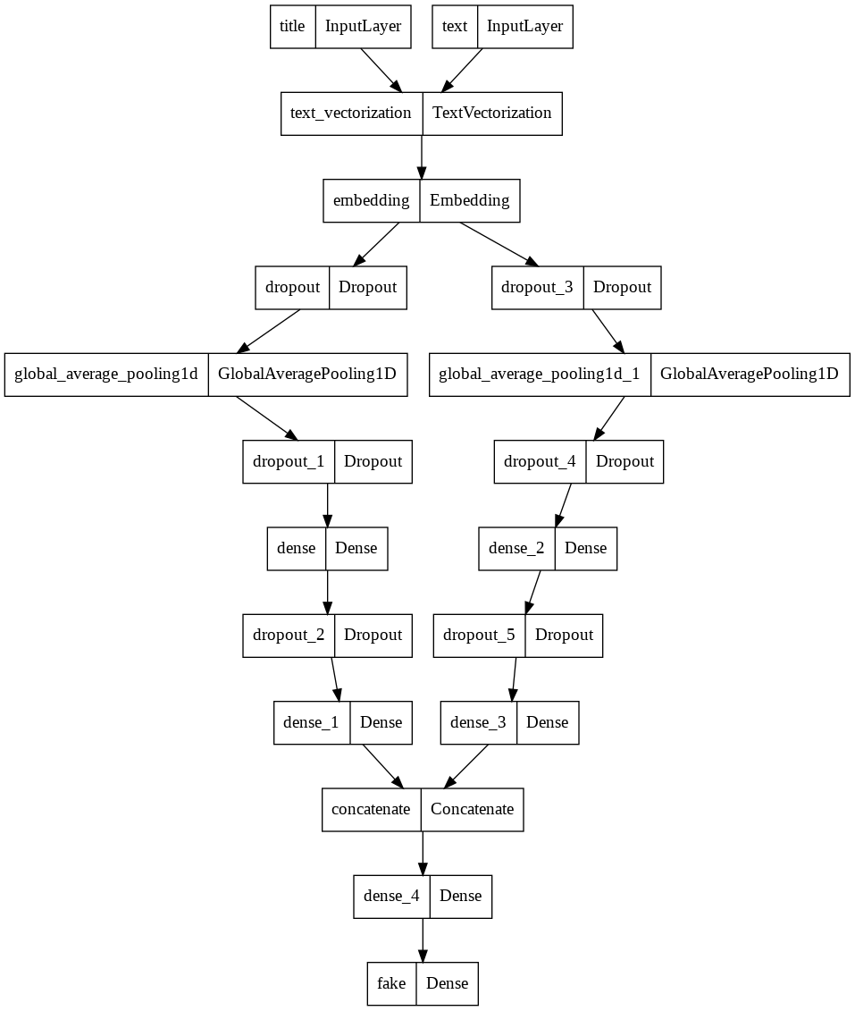
Finally, let’s compile and train the third model.

main_model.compile(optimizer = "adam",
              loss = losses.SparseCategoricalCrossentropy(from_logits=True),
              metrics=['accuracy']
)

main_history = main_model.fit(train_dataset, 
                              validation_data=val_dataset,
                              epochs = 30)

Click to show all 30 epochs from the third model.


    Epoch 1/30
    180/180 [==============================] - 5s 18ms/step - loss: 0.1592 - accuracy: 0.9398 - val_loss: 0.0293 - val_accuracy: 0.9918
    Epoch 2/30
    180/180 [==============================] - 3s 14ms/step - loss: 0.0472 - accuracy: 0.9835 - val_loss: 0.0314 - val_accuracy: 0.9924
    Epoch 3/30
    180/180 [==============================] - 3s 15ms/step - loss: 0.0413 - accuracy: 0.9873 - val_loss: 0.0253 - val_accuracy: 0.9947
    Epoch 4/30
    180/180 [==============================] - 3s 14ms/step - loss: 0.0405 - accuracy: 0.9865 - val_loss: 0.0167 - val_accuracy: 0.9962
    Epoch 5/30
    180/180 [==============================] - 3s 14ms/step - loss: 0.0386 - accuracy: 0.9871 - val_loss: 0.0178 - val_accuracy: 0.9967
    Epoch 6/30
    180/180 [==============================] - 3s 14ms/step - loss: 0.0370 - accuracy: 0.9877 - val_loss: 0.0242 - val_accuracy: 0.9944
    Epoch 7/30
    180/180 [==============================] - 3s 14ms/step - loss: 0.0335 - accuracy: 0.9887 - val_loss: 0.0379 - val_accuracy: 0.9798
    Epoch 8/30
    180/180 [==============================] - 3s 14ms/step - loss: 0.0336 - accuracy: 0.9891 - val_loss: 0.0470 - val_accuracy: 0.9756
    Epoch 9/30
    180/180 [==============================] - 3s 14ms/step - loss: 0.0303 - accuracy: 0.9893 - val_loss: 0.0134 - val_accuracy: 0.9973
    Epoch 10/30
    180/180 [==============================] - 3s 14ms/step - loss: 0.0290 - accuracy: 0.9909 - val_loss: 0.0292 - val_accuracy: 0.9882
    Epoch 11/30
    180/180 [==============================] - 3s 14ms/step - loss: 0.0280 - accuracy: 0.9908 - val_loss: 0.0345 - val_accuracy: 0.9827
    Epoch 12/30
    180/180 [==============================] - 3s 14ms/step - loss: 0.0289 - accuracy: 0.9902 - val_loss: 0.0344 - val_accuracy: 0.9827
    Epoch 13/30
    180/180 [==============================] - 3s 14ms/step - loss: 0.0245 - accuracy: 0.9928 - val_loss: 0.0160 - val_accuracy: 0.9951
    Epoch 14/30
    180/180 [==============================] - 3s 14ms/step - loss: 0.0247 - accuracy: 0.9913 - val_loss: 0.0196 - val_accuracy: 0.9933
    Epoch 15/30
    180/180 [==============================] - 3s 14ms/step - loss: 0.0251 - accuracy: 0.9914 - val_loss: 0.0290 - val_accuracy: 0.9854
    Epoch 16/30
    180/180 [==============================] - 3s 14ms/step - loss: 0.0270 - accuracy: 0.9920 - val_loss: 0.0509 - val_accuracy: 0.9724
    Epoch 17/30
    180/180 [==============================] - 3s 15ms/step - loss: 0.0263 - accuracy: 0.9918 - val_loss: 0.0345 - val_accuracy: 0.9844
    Epoch 18/30
    180/180 [==============================] - 3s 14ms/step - loss: 0.0260 - accuracy: 0.9908 - val_loss: 0.0440 - val_accuracy: 0.9764
    Epoch 19/30
    180/180 [==============================] - 3s 15ms/step - loss: 0.0252 - accuracy: 0.9915 - val_loss: 0.0171 - val_accuracy: 0.9933
    Epoch 20/30
    180/180 [==============================] - 3s 14ms/step - loss: 0.0232 - accuracy: 0.9925 - val_loss: 0.0246 - val_accuracy: 0.9878
    Epoch 21/30
    180/180 [==============================] - 3s 15ms/step - loss: 0.0255 - accuracy: 0.9911 - val_loss: 0.0294 - val_accuracy: 0.9858
    Epoch 22/30
    180/180 [==============================] - 3s 15ms/step - loss: 0.0204 - accuracy: 0.9935 - val_loss: 0.0225 - val_accuracy: 0.9916
    Epoch 23/30
    180/180 [==============================] - 3s 14ms/step - loss: 0.0203 - accuracy: 0.9925 - val_loss: 0.0286 - val_accuracy: 0.9860
    Epoch 24/30
    180/180 [==============================] - 3s 14ms/step - loss: 0.0199 - accuracy: 0.9935 - val_loss: 0.0201 - val_accuracy: 0.9907
    Epoch 25/30
    180/180 [==============================] - 4s 23ms/step - loss: 0.0205 - accuracy: 0.9928 - val_loss: 0.0151 - val_accuracy: 0.9947
    Epoch 26/30
    180/180 [==============================] - 3s 17ms/step - loss: 0.0216 - accuracy: 0.9924 - val_loss: 0.0506 - val_accuracy: 0.9753
    Epoch 27/30
    180/180 [==============================] - 3s 14ms/step - loss: 0.0223 - accuracy: 0.9925 - val_loss: 0.0241 - val_accuracy: 0.9889
    Epoch 28/30
    180/180 [==============================] - 3s 14ms/step - loss: 0.0224 - accuracy: 0.9915 - val_loss: 0.0547 - val_accuracy: 0.9780
    Epoch 29/30
    180/180 [==============================] - 3s 14ms/step - loss: 0.0224 - accuracy: 0.9911 - val_loss: 0.0551 - val_accuracy: 0.9771
    Epoch 30/30
    180/180 [==============================] - 3s 14ms/step - loss: 0.0212 - accuracy: 0.9924 - val_loss: 0.0303 - val_accuracy: 0.9856

Let’s plot the history of the accuracy on both the training and validation sets for the third model.

history_plot(main_history, model_name="Third Model")

blog post 6 model3 history

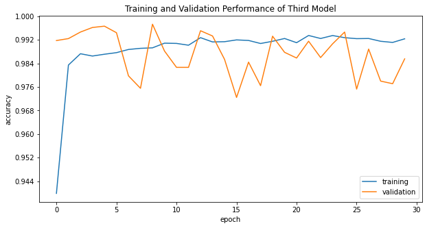
The third model consistently scores at least 97% validation accuracy in all epochs. Therefore, the third model is the best one. On the other hand, the second model, which only uses article title, consistently scores approximately 95% - 99% validation accuracy after epoch 14, which is also good.

As a result, using both the title of the article and the full text of the article is the most effective way to detect fake news. However, the third model is much more complicated and needs more time to train than the second model, and both models have a good performance. We might consider using the second model when we only have limited computing power and time.

§4. Model Evaluation

In this section we will download the test data, and test our model performance on unseen test data.

Don’t forget that we also need to convert the test dataframe to the dataset by using the function make_dataset().

test_url = "https://github.com/PhilChodrow/PIC16b/blob/master/datasets/fake_news_test.csv?raw=true"
test_df = pd.read_csv(train_url)
# conver to dataset
test_dataset = make_dataset(test_df)

Now, we can check our best model (the third model) performance on unseen data.

main_model.evaluate(test_dataset)

225/225 [==============================] - 3s 11ms/step - loss: 0.0284 - accuracy: 0.9864
[0.02836262620985508, 0.9864136576652527]

That’s impressive; the third model has almost 99% accuracy predicted if the article contains fake news.

Since our second model also performs well, let’s check its performance on unseen data too.

text_model.evaluate(test_dataset)

225/225 [==============================] - 3s 14ms/step - loss: 0.0606 - accuracy: 0.9710
[0.060581598430871964, 0.9710454940795898]

The result for the second model is almost 97% accuracy predicted if the article contains fake news.

Both the third and second models have an excellent performance. Therefore, we might consider using only the article’s full text to detect fake news when time is limited.

§5. Embedding Visualization

Word embeddings are often produced as intermediate stages in many machine learning algorithms. Let’s take a look at the embedding layer to see how our own model represents words in a vector space.

weights = main_model.get_layer('embedding').get_weights()[0] # get the weights from the embedding layer
vocab = vectorize_layer.get_vocabulary()                     # get the vocabulary from our data prep for later

Let’s check the shape of the weight

weights.shape

(2600, 3)

We have three columns because we set the output_dim = 3 in the embedding layer.

If we want to plot in 2-dimensional, we must reduce the weight from 3-dimensional into 2-dimensional by using the principal component analysis (PCA).

from sklearn.decomposition import PCA
pca = PCA(n_components=2)
weights = pca.fit_transform(weights)

Let’s double-check the shape of the weights.

weights.shape

(2600, 2)

Good, now we have successfully converted the weights from 3-dimensional into 2-dimensional.

Let’s make a dataframe from our results:

embedding_df = pd.DataFrame({
    'word' : vocab,         
    'x0'   : weights[:,0],   # zero column of the weights
    'x1'   : weights[:,1],   # first column of the weights
})

Let’s check our embedding_df.

embedding_df

	word	x0	x1
0		-0.009576	0.025002
1	[UNK]	-0.058210	0.053124
2	the	-0.387607	0.042387
3	to	0.051087	0.091192
4	of	0.302065	0.076064
...	...	...	...
2595	jury	-0.039374	-0.065970
2596	jackson	0.302881	-0.100250
2597	impossible	0.828751	-0.256427
2598	emerged	-0.646941	0.213412
2599	complained	0.178686	-0.326047

2600 rows × 3 columns

We have a special world UNK in our data frame. The first row in the word frequency is the unknown word that is not in the top 2600 words. So the most common word is the word does not actually on the list, which makes sense since those individual words it’s not common enough to make the top 2600, but if you add them all together and say they all count as an unknown word, added all together, they are going to be at the top rank.

Finally, we can make the plot.

fig = px.scatter(embedding_df, 
                 x = "x0", 
                 y = "x1", 
                 size = list(np.ones(len(embedding_df))),
                 size_max = 4,
                 hover_name = "word",
                 title='Embedding Visualization')
fig.update_layout(title_x=0.5)
                
fig.show()

On the left side, negativity x0 axis, we have words such as:

(-6.200, -0.175) : “gop” (the most left side word)
(-4.599, 0.192) : “watch”
(-4.208, -0.204) : “breaking”
(-4.091, 0.122). : “reportedly”
(-4.084, -0.241) : “rep”

On the right side, positive x0 axis, we have words such as:

(6.464, -0.206) : “trumps” (most right side word)
(4.420, -0.105) : “myanmar”
(4.210, -0.191) : “im”
(4.071, -0.058) : “dont”
(4.017, -0.143) : “rohingya”

I am not sure which side is more likely to be fake news, but there are more sensitive words on the left side, such as:

(-3.030,-0.074) : “racist”,
(-1.912,-0.156) : “conspiracy”
(-1.490,-0.175) : “hate”
(-1.159, 0.137) : “shooting”
(-0.727,-0.172) : “muslims”

Bias in Language Models

Bias is a common problem in language models, and bias can sneak into our language model. However, it does not require a biased modeler to create a biased model. It just requires a modeler who’s not being sufficiently careful.

Here we can learn about the possible biases learned by our model. Let’s check what kinds of words our model associated with females and males.

feminine = ["she", "her", "woman"]
masculine = ["he", "him", "man"]

highlight_1 = ["strong", "powerful", "smart",     "thinking"]
highlight_2 = ["hot",    "sexy",     "beautiful", "shopping"]

def gender_mapper(x):
    if x in feminine:
        return 1
    elif x in masculine:
        return 4
    elif x in highlight_1:
        return 3
    elif x in highlight_2:
        return 2
    else:
        return 0

embedding_df["highlight"] = embedding_df["word"].apply(gender_mapper)
embedding_df["size"]      = np.array(1.0 + 50*(embedding_df["highlight"] > 0))

fig = px.scatter(embedding_df, 
                 x = "x0", 
                 y = "x1", 
                 color = "highlight",
                 size = list(embedding_df["size"]),
                 size_max = 20,
                 hover_name = "word",
                 title='Embedding Visualization with Highlight')

fig.update_layout(title_x=0.5)

fig.show()

Written on March 3, 2022